Navigation :

Interference of two cosinoidal plane waves

Instead of only one plane wave, we simulate two different plane waves with different wave-vectors entering the simulation box, interfering and leaving the box again. In addition to the wave from the last tutorial, we add a second wave with different wave length, and entering the box at an angle, and shifted by 28 Bohr along the corresponding direction of propagation.

click for complete input


# ----- Calculation mode and parallelization ------------------------------------------------------

 CalculationMode                   = td
 ExperimentalFeatures = yes

 %Systems
   'Maxwell' | maxwell
 %

 Maxwell.ParDomains = auto
 Maxwell.ParStates  = no

# ----- Maxwell box variables ---------------------------------------------------------------------

 # free maxwell box limit of 10.0 plus 2.0 for the incident wave boundaries with
 # der_order = 4 times dx_mx

 lsize_mx = 12.0
 dx_mx    = 0.5

 Maxwell.BoxShape = parallelepiped

 %Maxwell.Lsize
  lsize_mx | lsize_mx | lsize_mx
 %

 %Maxwell.Spacing
  dx_mx | dx_mx | dx_mx
 %

# ----- Maxwell calculation variables -------------------------------------------------------------

 MaxwellHamiltonianOperator = faraday_ampere

 %MaxwellBoundaryConditions
  plane_waves | plane_waves | plane_waves
 %

 %MaxwellAbsorbingBoundaries
  not_absorbing | not_absorbing | not_absorbing
 %

# ----- Time step variables -----------------------------------------------------------------------

 TDSystemPropagator = exp_mid

 timestep = 1 / ( sqrt(c^2/dx_mx^2 + c^2/dx_mx^2 + c^2/dx_mx^2) )
 TDTimeStep                        = timestep
 TDPropagationTime                 = 150*timestep

# ----- Output variables --------------------------------------------------------------------------

 OutputFormat = plane_x + plane_y + plane_z + axis_x + axis_y + axis_z

# ----- Maxwell output variables ------------------------------------------------------------------

 %MaxwellOutput
  electric_field 
  magnetic_field 
  maxwell_energy_density 
  trans_electric_field
 %

 MaxwellOutputInterval             = 50
 MaxwellTDOutput                   = maxwell_energy + maxwell_total_e_field + maxwell_total_b_field

# ----- Maxwell field variables -------------------------------------------------------------------

 # laser propagates in x direction

 lambda1 = 10.0
 omega1  = 2 * pi * c / lambda1
 k1_x    = omega1 / c
 E1_z    = 0.05
 pw1     = 10.0
 ps1_x   = - 25.0

 # laser propagates in x-y direction

 alpha = pi/4
 lambda2 = 4.0
 omega2  = 2 * pi * c / lambda2
 k2_x    = omega2 / c * cos(alpha)
 k2_y    = omega2 / c * sin(alpha)
 E2_z    = 0.05
 pw2     = 10.0
 ps2_x   = - 28.0 * cos(alpha)
 ps2_y   = - 28.0 * sin(alpha)

 %MaxwellIncidentWaves
   plane_wave_mx_function | 0 | 0 | E1_z | "plane_waves_function_1"
   plane_wave_mx_function | 0 | 0 | E2_z | "plane_waves_function_2"
 %

 %MaxwellFunctions
   "plane_waves_function_1" | mxf_cosinoidal_wave | k1_x | 0    | 0 | ps1_x | 0     | 0 | pw1
   "plane_waves_function_2" | mxf_cosinoidal_wave | k2_x | k2_y | 0 | ps2_x | ps2_y | 0 | pw2
 %

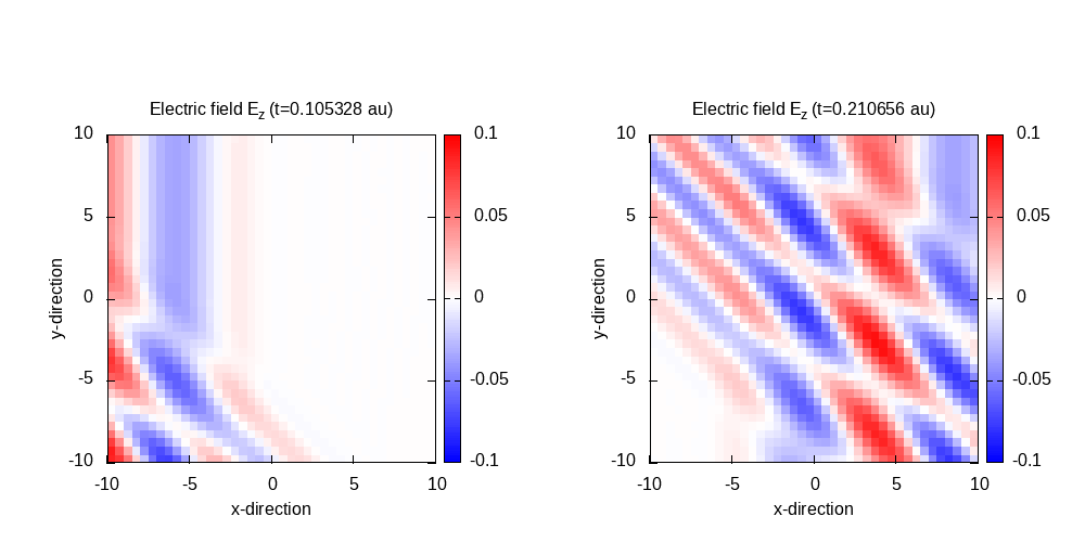
Both electric fields are polarized only in z-direction, and the magnetic field only in y-direction.

We can start from the last input file, and add the second wave, according to the following excerpt:


# ----- Maxwell field variables -------------------------------------------------------------------

 # laser propagates in x direction

 lambda1 = 10.0
 omega1  = 2 * pi * c / lambda1
 k1_x    = omega1 / c
 E1_z    = 0.05
 pw1     = 10.0
 ps1_x   = - 25.0

 # laser propagates in x-y direction

 alpha = pi/4
 lambda2 = 4.0
 omega2  = 2 * pi * c / lambda2
 k2_x    = omega2 / c * cos(alpha)
 k2_y    = omega2 / c * sin(alpha)
 E2_z    = 0.05
 pw2     = 10.0
 ps2_x   = - 28.0 * cos(alpha)
 ps2_y   = - 28.0 * sin(alpha)

 %MaxwellIncidentWaves
   plane_wave_mx_function | 0 | 0 | E1_z | "plane_waves_function_1"
   plane_wave_mx_function | 0 | 0 | E2_z | "plane_waves_function_2"
 %

 %MaxwellFunctions
   "plane_waves_function_1" | mxf_cosinoidal_wave | k1_x | 0    | 0 | ps1_x | 0     | 0 | pw1
   "plane_waves_function_2" | mxf_cosinoidal_wave | k2_x | k2_y | 0 | ps2_x | ps2_y | 0 | pw2
 %

Contour plot of the electric field in z-direction after 50 time steps for t=0.11 and 100 time steps for t=0.21:

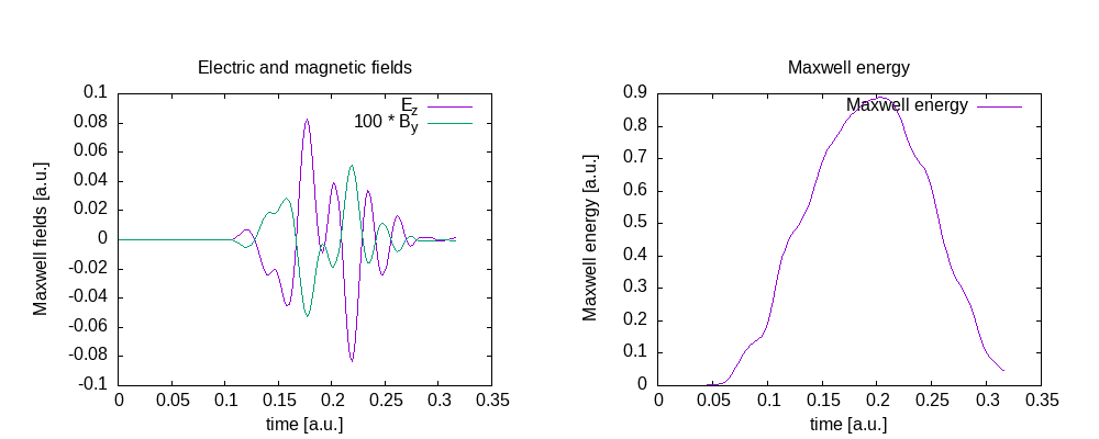
Maxwell fields at the origin and Maxwell energy inside the free Maxwell propagation region of the simulation box: