Non-dispersive linear media
Including non-disperive linear media objects
An arbitrary number of linear medium shapes can be placed inside simulation box. Linear media are defined as a separate system type, for example:
%Systems
 'Maxwell' | maxwell
 'Medium'  | linear_medium
%
The object shape can be defined in two ways, which are given by the variable
LinearMediumBoxShape: if set to medium_parallelepiped, the
parallelepiped box will be defined by its center, and size in each dimension
through the LinearMediumBoxSize block; if the box shape is
defined as medium_box_file, the box shape will be read from an external
geometry file in OFF format,
defined through the variable LinearMediumBoxFile.
In this tutorial, we will simulate light propagation though a spherical lens,
for which we need to provide an OFF file representing a suitable shape. There
are many software packages around to generate such files, but we recommend
openSCAD and ctmconv which is part
of OpenCTM.
In Debian style systems, these can be installed using
    apt-get install openscad
    apt-get install openctm-tools
OpenSCAD provides its own scripting language for creating geometries, which can be created in a GUI, but also can be rendered on the command line. Here we will use the following code to create a simple lens from the intersection of two spheres and shift its position to the negative x-axis with openSCAD, using the following script:
$fs=2.0;
$fa=2.0;
translate([-10,0,0]) {
intersection(){
  translate([-8,0,0]) sphere(r=10);
  translate([ 8,0,0]) sphere(r=10);
};
};
copy the above code into a file lens.scad, you can generate the required
OFF file by the command:
openscad -o lens.off lens.scad
For details on the syntax of this, see the openSCAD tutorials.
This creates the following lens: 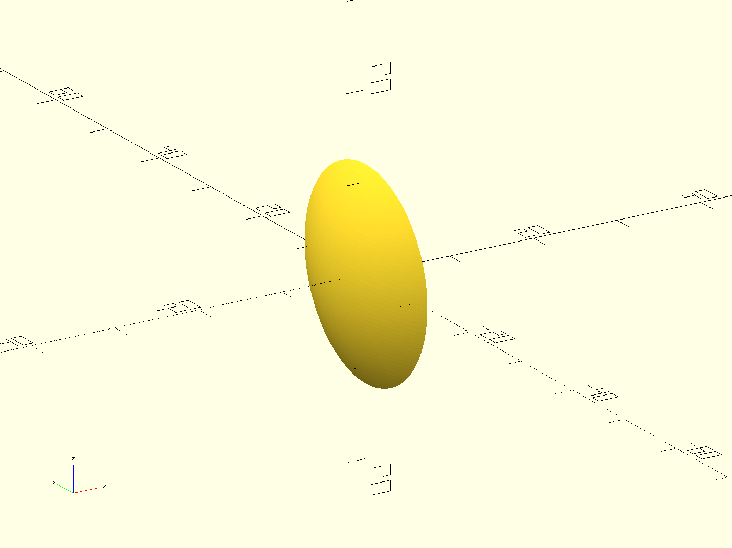
Now we have the OFF file, let’s consider the
electromagnetic properties of the medium. These must be defined in the LinearMediumProperties block, which specifies the relative electric
permittivity, relative magnetic permeability, and the electric and magnetic
conductivities (for lossy media). In addition to
adding the linear_medium system, we need to switch the MaxwellHamiltonianOperator to faraday_ampere_medium.
As a linear medium will scatter waves in all directions, there need to be
absorbing boundary conditions to avoid spurious reflections on the box
boundaries. For this purpose, we change the MaxwellAbsorbingBoundaries block to mask in all directions, to damp the
field at the boundaries by multiplying it with a scalar mask function. The
width of this mask MaxwellABMaskWidth is set to 5 Bohr.
As a consequence of the additional region for the absorbing boundary condition,
we have to increase the box size. Therefore, the lsize_mx value is
now 20.0 (13.0 Bohr for propagation region plus 2.0 Bohr for the incident wave
boundaries plus 5.0 Bohr for absorbing boundary conditions).
Finally, as non-dispersive linear media are static,
TDSystemPropagator = static
, which is the default option, must be set for the medium,
while the Maxwell system needs to be set to exp_mid. A possible
input file to run this simulation, then, would be the following:
CalculationMode = td
ExperimentalFeatures = yes

%Systems
 'Maxwell' | maxwell
 'Medium'  | linear_medium
%

Maxwell.ParDomains = auto
Maxwell.ParStates  = no

# free maxwell box limit of 13.0 plus 2.0 for the incident wave boundaries with
# der_order times dx_mx (here: der_order = 4) plus 5.0 for absorbing boundary conditions

lsize_mx = 20.0
dx_mx    = 0.5

BoxShape = parallelepiped

%Lsize
 lsize_mx | lsize_mx | lsize_mx
%

%Spacing
 dx_mx | dx_mx | dx_mx
%

LinearMediumBoxShape = medium_box_file
LinearMediumBoxFile = "lens.off"
%LinearMediumProperties
 5.0 | 1.0 | 0.0 | 0.0
%

MaxwellHamiltonianOperator = faraday_ampere_medium

%MaxwellBoundaryConditions
 plane_waves | plane_waves | plane_waves
%

%MaxwellAbsorbingBoundaries
 mask | mask | mask
%

MaxwellABWidth = 5.0

Maxwell.TDSystemPropagator = exp_mid

timestep = 1 / ( sqrt(c^2/dx_mx^2 + c^2/dx_mx^2 + c^2/dx_mx^2) )
Maxwell.TDTimeStep = timestep
Medium.TDTimeStep = timestep/2
TDPropagationTime = 150*timestep

OutputFormat = plane_x + plane_y + plane_z + axis_x + axis_y + axis_z

%MaxwellOutput
 electric_field
%

MaxwellOutputInterval = 25
MaxwellTDOutput = maxwell_energy + maxwell_total_e_field + maxwell_total_b_field


lambda1 = 10.0
omega1  = 2 * pi * c / lambda1
k1_x    = omega1 / c
E1_z    = 0.05
pw1     = 10.0
ps1_x   = - 25.0

# laser propagates in x direction
%MaxwellIncidentWaves
  plane_wave_mx_function | 0 | 0 | E1_z | "plane_waves_function_1"
%

%MaxwellFunctions
  "plane_waves_function_1" | mxf_cosinoidal_wave | k1_x | 0    | 0 | ps1_x | 0     | 0 | pw1
%
As the exp_mid propagator contains two algorithmic steps, it must
be clocked twice as fast as the static propagator and hence the
time step of the medium bust be set to half the Maxwell time step. This is
currently a workaround, and is likely to change in future releases of the code.
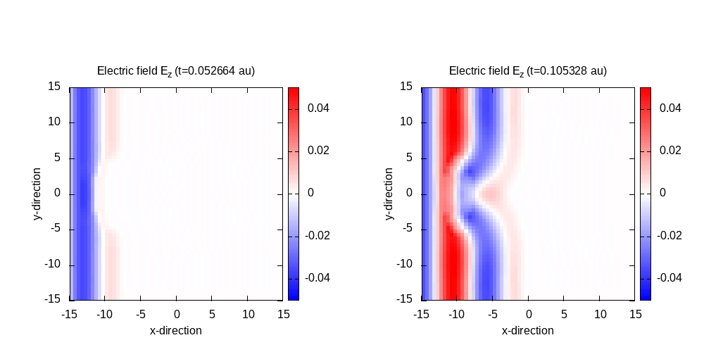
For this run, we use the previous incident plane wave propagating only in the x-direction but place a medium box inside the simulation box. After running the code, we can visualize the results with the following gnuplot script:
Contour plot of the electric field in z-direction after 50 time steps for
t=0.11 and 100 time steps for t=0.21:
Contour plot of the electric field in z-direction after 125 time steps for
t=0.26 and 150 time steps for t=0.32:
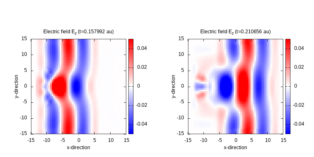
In the last panel, it can be seen that there is a significant amount of scattered waves which, in large parts, are scattered from the box boundaries. This is due to making use of plane wave boundary conditions and absorbing boundaries simultaneously, and would be less noticeable if we increase the size of the box. In this tutorial we keep the box small to stay within a reasonable computation time.