External currents and PML
External current density
Not absorbing boundaries
Instead of an incoming external plane wave, Octopus can simulate also external current densities placed inside the simulation box. In this example we place an array of such current densities in the simulation box and study the properties of the emitted field and the effect of the absorbing boundaries.
Since we start with no absorbing boundaries, we set the box size to 10.0.
CalculationMode   = td
ExperimentalFeatures = yes
FromScratch = yes

%Systems
  'Maxwell' | maxwell
%
lsize_mx = 10.0
dx_mx    = 0.5

%Maxwell.Lsize
 lsize_mx | lsize_mx | lsize_mx
%

%Maxwell.Spacing
 dx_mx | dx_mx | dx_mx
%

%MaxwellBoundaryConditions
 zero | zero | zero
%

%MaxwellAbsorbingBoundaries
 not_absorbing | not_absorbing | not_absorbing
%

OutputFormat = axis_x + plane_x + plane_y + plane_z
MaxwellOutputInterval = 10
MaxwellTDOutput       = maxwell_energy + maxwell_total_e_field

%MaxwellOutput
 electric_field
 magnetic_field
 maxwell_energy_density
 external_current | "output_format" | plane_z | "output_interval" | 2
%

%MaxwellFieldsCoordinate
 0.00 | 0.00 | 0.00
%

TDSystemPropagator = exp_mid
timestep           = 1 / ( sqrt(c^2/dx_mx^2 + c^2/dx_mx^2 + c^2/dx_mx^2) )
TDTimeStep         = timestep
TDPropagationTime  = 180 * timestep

ExternalCurrent = yes
t1 = (180 * timestep) / 2
tw = (180 * timestep) / 6
j = 1.0000
sigma = 0.5
lambda = 5.0
omega = 2 * pi * c / lambda

%UserDefinedMaxwellExternalCurrent
 current_td_function | "0" | "0" | "j*exp(-(x+8)^2/2/sigma^2)*exp(-(y-5)^2/2/sigma^2)*exp(-z^2/2/sigma^2)" | omega | "env_func_1"
 current_td_function | "0" |" 0" | "j*exp(-(x+8)^2/2/sigma^2)*exp(-y^2/2/sigma^2)*exp(-z^2/2/sigma^2)"     | omega | "env_func_1"
 current_td_function | "0" | "0" | "j*exp(-(x+8)^2/2/sigma^2)*exp(-(y+5)^2/2/sigma^2)*exp(-z^2/2/sigma^2)" | omega | "env_func_1"
%

%TDFunctions
 "env_func_1" | tdf_gaussian | 1.0 | tw | t1
%
The external current density is switched on by the corresponding options and two blocks define its spatial distribution and its temporal behavior. In this example we place three sources, located near the box boundary in the negative x direction, and separated by 5 bohr along the y axis. As all of them are polarized in the z direction, only the z component is non zero. The spatial distribution of our example external current sources is a Gaussian distribution in 3D. The temporal pulse is a sinusoidal wave with a wavelength of 5 bohr, modulated by a Gaussian envelope centered at half the total simulation time, and with a variance $\sigma^2$ of 0.25.
ExternalCurrent = yes
t1 = (180 * timestep) / 2
tw = (180 * timestep) / 6
j = 1.0000
sigma = 0.5
lambda = 5.0
omega = 2 * pi * c / lambda

%UserDefinedMaxwellExternalCurrent
 current_td_function | "0" | "0" | "j*exp(-(x+8)^2/2/sigma^2)*exp(-(y-5)^2/2/sigma^2)*exp(-z^2/2/sigma^2)" | omega | "env_func_1"
 current_td_function | "0" |" 0" | "j*exp(-(x+8)^2/2/sigma^2)*exp(-y^2/2/sigma^2)*exp(-z^2/2/sigma^2)"     | omega | "env_func_1"
 current_td_function | "0" | "0" | "j*exp(-(x+8)^2/2/sigma^2)*exp(-(y+5)^2/2/sigma^2)*exp(-z^2/2/sigma^2)" | omega | "env_func_1"
%

%TDFunctions
 "env_func_1" | tdf_gaussian | 1.0 | tw | t1
%
In addition to the electric field and energy density, we set the external current as output, to visualize the shape and temporal profile and check that our input file is correct. As we want a more frequent output for this quantity, and only the z=0 plane output is sufficient, we select a specific output format and interval for this quantity only. For the other quantities, the global formats and interval apply.
OutputFormat = axis_x + plane_x + plane_y + plane_z
MaxwellOutputInterval = 10
MaxwellTDOutput       = maxwell_energy + maxwell_total_e_field

%MaxwellOutput
 electric_field
 magnetic_field
 maxwell_energy_density
 external_current | "output_format" | plane_z | "output_interval" | 2
%
After running Octopus, we first visualize the current pulse using the following gnuplot script.
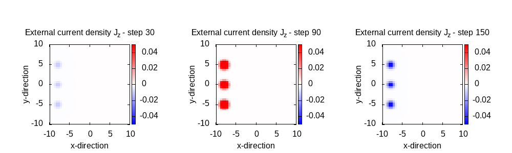
We observe the three sources with their Gaussian spatial profile. Now, to see the temporal profile, we extract the value of the current density at one specific point, namely (-8 Bohr, 0, 0), from all of the output files. Inspecting one of the output_iter/td.*/external_current-z.z=0 files, we find that the aforementioned point corresponds to line 195, and the field value is in column 3. Then, to grab these numbers for all time steps, we can run this simple bash command:
for td in Maxwell/output_iter/td.0000*; do jj=$(sed -n '195p' $td//external_current-z.z\=0 | awk {'print $3'}); tdi=${td:27:6}; echo $tdi $jj >> current_vs_t.dat; done
This creates a file with the time step number in the first column, and the value of the current in the second column. In order to plot this, we can use gnuplot:

The EM irradiated by these current pulses should look like plane waves far enough from the sources, and should have the same temporal profile than the source. Let’s look at the total electric field at the origin of the box, that is printed to Maxwell/td.general/total_e_field_z:
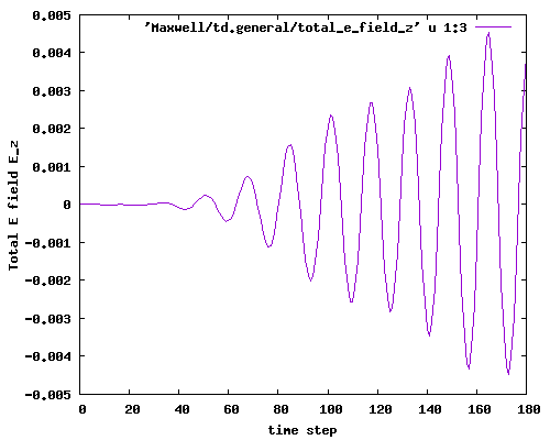
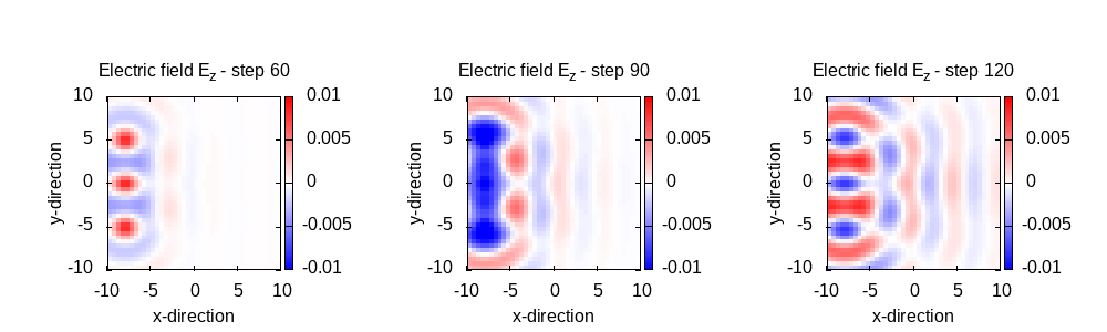
Clearly the amplitude increases and does not have a Gaussian envelope. Let’s inspect the E field in the z=0 plane to understand why, using the following plotting script:
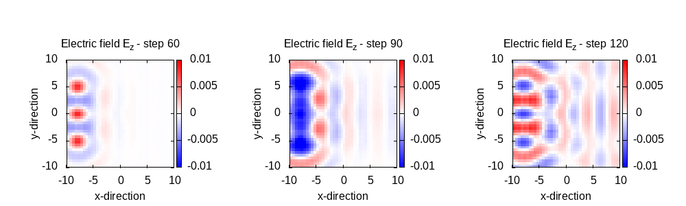
After step 90 we start seeing a strong effect from the reflections that occur at the box boundaries. In the following, we activate the PML boundary conditions to improve this behaviour.
PML absorbing boundaries
Taking the previous input file as template, we now modify the absorbing boundaries block:
 %MaxwellAbsorbingBoundaries
  cpml | cpml | cpml
 %

 MaxwellABWidth = 5.0
We set a boundary width of 5 Bohr (it should be at least 8 grid points, which according to our spacing, would be 4 Bohr). With this additional absorbing width, we have to update the simulation box dimensions.
 lsize_mx = 15.0
 dx_mx    = 0.5

 %Maxwell.Lsize
  lsize_mx | lsize_mx | lsize_mx
 %
The rest of the input options remain the same. After running the code, we now check the temporal profile of the E field at the box center, plotting again column 3 vs. column 1 of the file Maxwell/td.general/total_e_field_z using the same script as before:
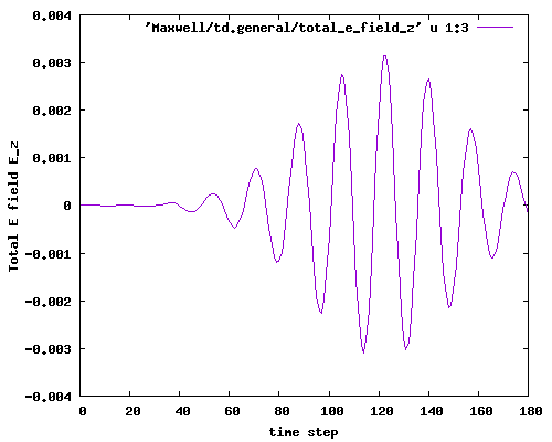
Now we do observe the Gaussian envelope. Looking at the z=0 plane E field, (plotting it with the same script as before) we confirm the reflection problem is gone:
Assignment:
- Is the E field only z-polarized? Check the other polarization directions.
- In which direction is the B field predominantly polarized?
- How much does the generated E_z field differ from a plane wave in the axis x = 8 Bohr? Grab the necessary data from the output files.