Wannier90
Starting from Octopus Selene (10.x), Octopus provides an interface for Wannier90. In order to perform this tutorial, you need first to compile Wannier90. Detailed information can be found on the Wannier90 website .
In this tutorial, we follow the second example from the Wannier90 tutorials, which consists in computing the Fermi surface of lead. This requires several steps, which are explained in detail bellow.
Ground-state
Input
We start with the input file for Octopus. At this point there is nothing special to specify as Octopus does not need to know that Wannier90 will be called later.
 CalculationMode = gs
 PeriodicDimensions = 3

 Spacing = 0.4

 %LatticeVectors
   0.0 | 0.5 | 0.5
   0.5 | 0.0 | 0.5
   0.5 | 0.5 | 0.0
 %

 a = 9.3555
 %LatticeParameters
  a | a | a
 %

 PseudopotentialSet = hgh_lda
 %ReducedCoordinates
  "Pb" | 0.0 | 0.0 | 0.0
 %

 %KPointsGrid
   4 |  4 |  4
 %

 Smearing = 0.1*eV
 SmearingFunction = fermi_dirac
 ExtraStates = 4
The use of most of these variables is already explained in detail in other tutorials. See, for example, the Periodic Systems tutorial. Nevertheless, some options deserve a more detailed explanation:
- SmearingFunction = fermi_dirac: as we are interested in lead, which is a metal, we need to use a smearing of the occupations in order to get a converged ground-state. Here we have chosen the smearing function to be a Fermi-Dirac distribution.
- Smearing = 0.1*eV: this defines the effective temperature of the smearing function.
- PseudopotentialSet = hgh_lda: since lead is not provided with the default pseudopotential set, we must select one containing Pb. We thus use the LDA HGH pseudopotential set here.
It is also important to note that the ‘‘k’'-point symmetries cannot be used with Wannier90. Also, only Monkhorst-Pack grids are allowed, so that only one ‘‘k’'-point shift is allowed.
Output
Now run Octopus using the above input file. The output should be similar to other ground-state calculations for periodic systems, so we are not going to look at it in detail. Nevertheless, to make sure there was no problem with the calculation and since we will need this information later, you should check the calculated Fermi energy. You can find this information in the static/info file:
Fermi energy = 0.157425 H
Wannier90
The usage of Wannier90 as a post-processing tool requires several steps and several invocations of both Wannier90 and Octopus. Note that all the interfacing between Wannier90 and Octopus is done through a specialized utility called oct-wannier90 .
Step one: create the Wannier90 input file
In order to run Wannier90, you must prepare an input file for it. To make this task easier, the oct-wannier90 utility can take the Octopus input file and “translate” it for Wannier90. Here is how the input file for the utility should look like:
 CalculationMode = gs
 PeriodicDimensions = 3

 Spacing = 0.4

 %LatticeVectors
   0.0 | 0.5 | 0.5
   0.5 | 0.0 | 0.5
   0.5 | 0.5 | 0.0
 %

 a = 9.3555
 %LatticeParameters
  a | a | a
 %

 PseudopotentialSet = hgh_lda
 %ReducedCoordinates
  "Pb" | 0.0 | 0.0 | 0.0
 %

 %KPointsGrid
   4 |  4 |  4
 %

 Smearing = 0.1*eV
 SmearingFunction = fermi_dirac
 ExtraStates = 4

 Wannier90Mode = w90_setup
This is basically the same input file as above with the following option added:
- Wannier90Mode = w90_setup: this tells the oct-wannier90 utility that we want to setup an input file for Wannier90 based on the contents of our input file.
Now run the the oct-wannier90 utility. This will create a file named w90.win that should look like this:
- this file has been created by the Octopus wannier90 utility

begin unit_cell_cart
Ang
   0.00000000   2.47535869   2.47535869
   2.47535869   0.00000000   2.47535869
   2.47535869   2.47535869   0.00000000
end unit_cell_cart

begin atoms_frac
Pb     0.00000000   0.00000000   0.00000000
end atoms_frac

use_bloch_phases = .true.

num_bands    6
num_wann    6

write_u_matrices = .true.
translate_home_cell = .true.
write_xyz = .true.

mp_grid    4   4   4

begin kpoints
 -0.00000000  -0.00000000  -0.00000000
 -0.25000000  -0.00000000  -0.00000000
...
Before running Wannier90, we are going to slightly tweak this file. As we are interested in lead, we will replace the following lines:
use_bloch_phases = .true.

num_bands    6
num_wann    6
by
num_bands    6
num_wann    4
begin projections
Pb:sp3
end projections
By doing this, we are telling Wannier90 that we want to find 4 Wannier states out of the 6 bands contained in the DFT calculation. Moreover, we are using guess projections based on sp3 orbitals attached to the lead atom. More details about Wannier90, projections, and disentanglement can be found in the tutorials and manual of Wannier90.
Step 2: generate the .nnkp file
After editing the file w90.win
, run Wannier90 in post-processing mode:
wannier90.x -pp w90.win
This will produce a file named w90.nnkp . This file contains information telling Octopus what further information does Wannier90 require for the following steps.
Step 3: generate files for Wannier90
At this stage, we are going to tell Octopus to generate some files for Wannier90 using the information from the w90.nnkp file. To do so, we change the value of the Wannier90Mode variable in the above Octopus input file to:
Wannier90Mode = w90_output
Step 4: run Wannier90
Finally, you call Wannier90 to perform the Wannierization:
wannier90.x w90.win
Computing the Fermi surface
Once you performed all the previous steps, you know how to run Wannier90 on top of an Octopus calculation. Lets now compute the interpolated Fermi surface. To do that, we add the following lines to the w90.win file:
restart = plot
fermi_energy = 4.283754645
fermi_surface_plot = true
The value of the Fermi energy corresponds to the one obtained by Octopus, converted to eV.
By calling again Wannier90, you will obtain a file w90.bxsf
, which you can plot using, for instance, xcrysden:
xcrysden --bxsf w90.bxsf
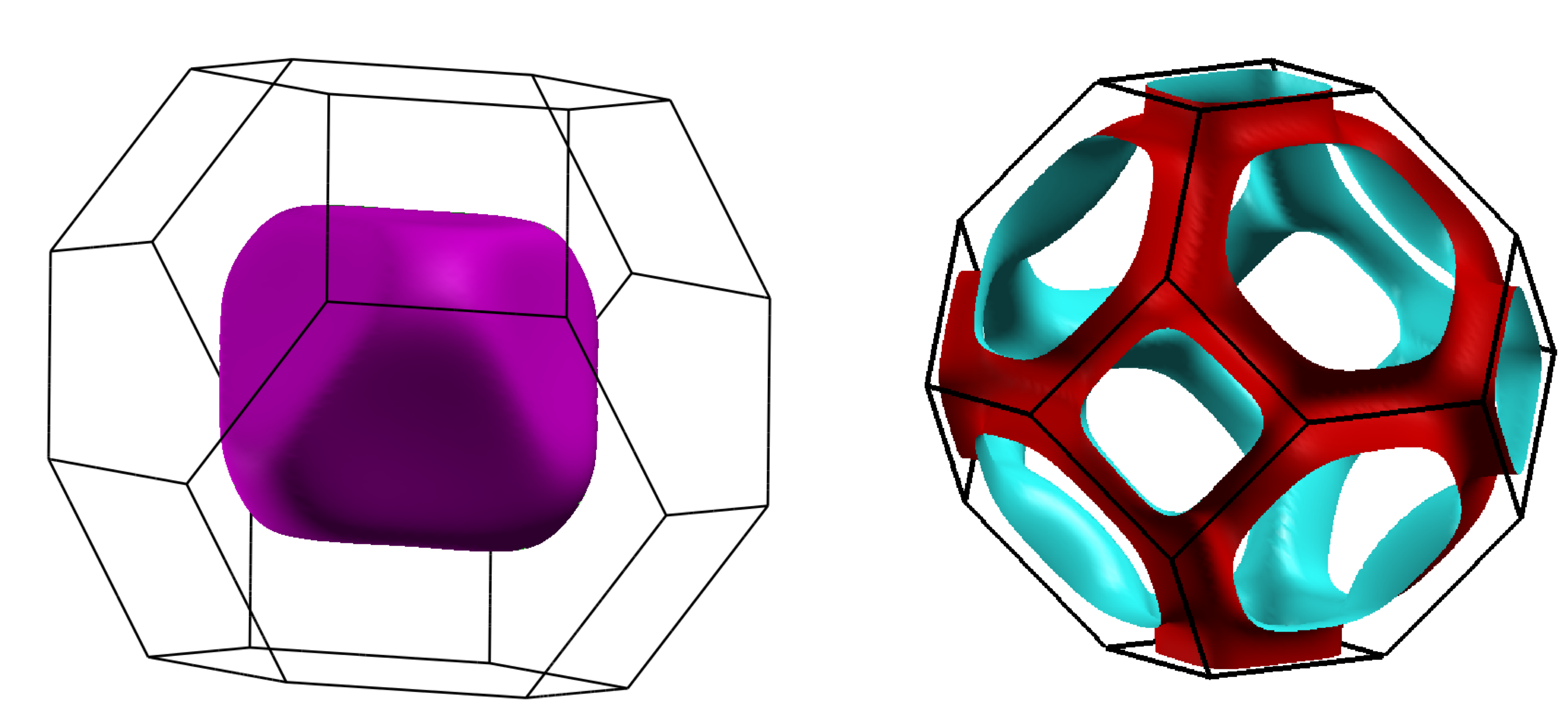
From here you should be able to produce the plot of the Fermi surface for band 2 and band 3, as shown in the figure.
Visualization of Wannier states using Octopus or Wannier90
Wannier90 allows one to compute the Wannier states. For this, you need to output the periodic part of the Bloch states on the real-space grid. This produces the .unk files. For this, you need to specify the output of oct-wannier90 by adding the following line to the inp file
Wannier90Files = w90_unk
Note that in order to get all the files you need in one run, you could instead use Wannier90Files = w90_amn + w90_mmn + w90_eig + w90_unk.
An alternative way of getting the states is to let Octopus compute them. You need to get the U matrices from Wannier90 for this by adding the following line to the w90.win file:
write_u_matrices = .true.
Then run the oct-wannier90 utility with the appropriate mode
Wannier90Mode = w90_wannier