ARPES
This tutorial aims at introducing the user to the basic concepts needed to calculate ARPES with Octopus. We choose as test case a fictitious non-interacting two-dimensional system with semi-periodic boundary conditions.
Ground state
Before starting with the time propagation we need to obtain the ground state of the system.
To simulate ARPES simulations with the tSURRF implementation in Octopus1 one needs to explicitly model the surface of the material. This requirement often leads to heavy simulations. For this reason, in this tutorial, we illustrate the procedure on a model system. Calculating ARPES with TDDFT on an ab-initio model for a surface involves the same steps.
Input
The system we choose is a 2D toy model potential simulating an atomic chain. The dimensionality is selected by telling octopus to use on 2 spatial dimensions (xy)
with Dimensions = 2 and by imposing periodic boundary conditions along x with
PeriodicDimensions = 1.
CalculationMode = gs
ExperimentalFeatures = yes

TheoryLevel = independent_particles
Dimensions = 2
PeriodicDimensions = 1

BoxShape = parallelepiped
Spacing = 0.5

LL = 120

%LatticeParameters
  8.15| LL
%

%LatticeVectors
  1.  | 0.
  0.  | 1.
%

U0 = 0.78
x0 = 0.565*1.88
y0 = 0.0


%Species
  "tanh" | species_user_defined | potential_formula | " -U0*(1+tanh(x+x0))*(1+tanh(x0-x))*(1+tanh(y+y0))*(1+tanh(-y+y0))" | valence | 4
%

%Coordinates
  "tanh" |   0.0   | 0.0
%


  %KpointsGrid
    1 | 1
  %

%KPointsPath
  20
  -0.5| 0
  0.5 | 0
%
Octopus can calculate ARPES on a path in reciprocal space. For this reason we have to specify the path with the KPointsPath block already at the ground state level. This is needed to generate the KS wave functions that will be evolved in the time propagation. It also provides the bands structure that we will use as reference to cross-check the quality of the spectrum.
Note that, since this is a toy model with independent electrons, TheoryLevel = independent_particles,
we do not need to sample the BZ and the grid in reciprocal space is constituted only by the gamma point,
  %KpointsGrid
    1 | 1
  %
Time-dependent run
To calculate the ARPES spectrum we excite the system with a laser field to excite electrons into the vacuum, i.e. on the non-periodic dimension. The photoelectron detection probability constituting ARPES is calculated by analyzing the flux of the ionization current trough a surface positioned at a certain distance from the surface of the system. This current is obtained by propagating in time the KS orbitals under the effect of the laser.
Input
This is how the input file should look for the time propagation.
Where we just changed the CalculationMode to td to activate the time propagation.
CalculationMode = td
We then have to specify the laser field parameters as following.
wpr = 52*eV            # Laser Frequency
II = 1.0E9             # Laser intensity in W/cm^2
EE = sqrt(II/3.51e+16) # Electric field peak amplitude
AApr = EE * 137/wpr    # Vector potential amplitude
TT = 10 * femtosecond  # Pulse envelope
tcpr= 2 * pi/wpr       # Field cycle
npr = TT/tcpr          # Number of cycles
Tpr = tcpr*npr         # Total pulse time
Since we deal with periodic system we have to specify the light-matter coupling in the so called “velocity gauge” where the field is described by a time-dependent vector potential. We specify the field as a “vector_potential” polarized along x and with carrier frequency “wpr”
%TDExternalFields
  vector_potential | 1  | 0  | 0 | wpr |"probe"
%
and a sin^2 envelope function “probe” specified by an analytical expression of time, t.
%TDFunctions
  "probe"  | tdf_from_expr | 'AApr*sin(wpr*(t)/(2*npr))^2*step(Tpr-(t))*step(t)'
%

TDTimeStep = 0.2
TDPropagationTime = Tpr
We also specified the total time of the propagation to be exactly synchronized with the pulse switch-off time by setting
TDPropagationTime = Tpr.
For more details look at the Time-dependent propagation tutorial.
Photoelectrons ejected from the system by the laser will eventually bounce back from the boundary of the simulation box along the non-periodic dimension (y). We therefore employ absorbing boundary conditions to prevent spurious reflections with the following code block
Lmin = 30

AbsorbingBoundaries = cap
ABCapHeight = -1.0
%ABShape
 Lmin | LL | "abs(y)"
%
Here we employ complex absorbing potential (CAP) boundaries with AbsorbingBoundaries = cap,
specify the CAP parameters ABCapHeight and ABShape to have maximal absorption in the energy region where we expect the photoelectrons.2
Finally we specify the parameters for the evaluation of the ARPES spectrum.
PhotoElectronSpectrum = pes_flux

PES_Flux_Lsize = Lmin

Emin =  wpr - 0.2
Emax =  wpr
DE   = 0.01
%PES_Flux_EnergyGrid
  Emin | Emax | DE
%
Here we tell octopus to use tSURFF with PhotoElectronSpectrum = pes_flux ,
specify the position of the analyzing surface at the onset of the absorbing boundaries with
PES_Flux_Lsize = Lmin and define the parameters of the energy grid for the
final spectrum with the block PES_Flux_EnergyGrid.
The tSURFF method allows to calculate the momentum-resolved photoelectron probability $P({\bf p})$ on an arbitrary grid in momentum space.
The ARPES spectrum is than obtained rewriting $P({\bf p})$ as a function of the total kinetic energy and the momentum parallel to the surface, ${\bf p}_\parallel$
(equivalent to the crystal momentum ${\bf k}$ ) $P({\bf p}_\parallel={\bf k}, E=({\bf p}_\parallel + {\bf p}_\perp)^2/2)$.
Since a simple cartesian grid in momentum results in a deformed ARPES grid octopus can generate a grid that compensates the deformation such the final ARPES spectrum is in a cartesian grid.
This grid is generated with PES_Flux_ARPES_grid = yes.
Since this option is true by default for semi-periodic systems we do not have to specify it in the input file.
Output
If the code runs correctly the standard output should present a Photoelectron section like this:
*************************** Photoelectron ****************************
Info: Calculating PES using t-surff technique.
Input: [PES_Flux_Shape = pln]
Input: [PES_Flux_Lsize = (8.150,30.00)]
Input: [PES_Flux_Parallelization = pf_none]
Input: [PES_Flux_Momenutum_Grid = cartesian]
Energy grid (Emin, Emax, DE) [H]:  (   1.711,   1.911, 0.10E-01)
Momentum linear grid (Pmin, Pmax, DP) [me*bH(2pi/h)]:  (   1.850,   1.955, 0.14E+00)
Input: [PES_Flux_ARPES_grid = yes]
Number of points with E < p//^2/2 = 0 [of 462]
Input: [PES_Flux_UseSymmetries = no]
Input: [PES_Flux_RuntimeOutput = no]
Info: Total number of surface points = 16
Info: Total number of momentum points = 21
ARPES
The spectral information on the photoelectrons is stored in restart/td/pesflux* binary files and can be analyzed in post-processing.
The oct-photoelectron_spectrum utility
Octopus provides an utility called oct-photoelectron_spectrum to process the pesflux* files and obtain the spectrum.
Input
The utility by default requires no input from the user in calculations designed to obtain an ARPES spectrum. If the td run has been performed with
PES_Flux_ARPES_grid = yes it should have all the information that it needs.
Just run the utility in the same path where the inp file resides.
Output
This is what you should get:
************************** Kpoint selection **************************
Will use a zero-weight path in reciprocal space with the following points
       2    0.000000 |   -0.500000    0.000000 |
       3    0.000000 |   -0.450000    0.000000 |
       4    0.000000 |   -0.400000    0.000000 |
       5    0.000000 |   -0.350000    0.000000 |
       6    0.000000 |   -0.300000    0.000000 |
       7    0.000000 |   -0.250000    0.000000 |
       8    0.000000 |   -0.200000    0.000000 |
       9    0.000000 |   -0.150000    0.000000 |
      10    0.000000 |   -0.100000    0.000000 |
      11    0.000000 |   -0.050000    0.000000 |
      12    0.000000 |    0.000000    0.000000 |
      13    0.000000 |    0.050000    0.000000 |
      14    0.000000 |    0.100000    0.000000 |
      15    0.000000 |    0.150000    0.000000 |
      16    0.000000 |    0.200000    0.000000 |
      17    0.000000 |    0.250000    0.000000 |
      18    0.000000 |    0.300000    0.000000 |
      19    0.000000 |    0.350000    0.000000 |
      20    0.000000 |    0.400000    0.000000 |
      21    0.000000 |    0.450000    0.000000 |
      22    0.000000 |    0.500000    0.000000 |

**********************************************************************

Read PES restart files.
Zenith axis: (      0.00,       0.00,       1.00)
[ 42/ 42] 100%|****************************************|     --:-- ETA

***************** ARPES cut on reciprocal space path *****************
Done
**********************************************************************
If all goes well the file is PES_ARPES.path will be created containing the ARPES spectrum evaluated on the k-point path. The spectrum can be visualized with gnuplot as a density plot with
set pm3d map
sp "PES_ARPES.path" u 1:4:5
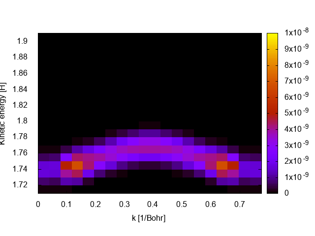
The ARPES spectrum looks a bit blocky to improve the resolution one has to increase the number of kpoints in “KPointsPath” (requires recomputing the groundstate) and decrease the energy spacing in PES_Flux_EnergyGrid. Keep in mind that larger grids implies heavier simulations and longer run times.
Some questions to think about:
-
How does the ARPES spectrum compares with the band structure? Plot one on top of the other with gnuplot .
-
How to choose the photoelectron energy range? In the previous example we chose Emin = wpr - 0.2 and Emax = wpr in order to see photoelectrons emitted from the valence band. How can we change PES_Flux_EnergyGrid to see the band below? What about conduction band?
-
Play around with the laser carrier, “wpr”, and pulse envelope, “Tpr”. Can you identify the impact of these parameters on the spectrum?
References
-
U. De Giovannini, H. Hübener, and A. Rubio, A First-Principles Time-Dependent Density Functional Theory Framework for Spin and Time-Resolved Angular-Resolved Photoelectron Spectroscopy in Periodic Systems, JCTC 13 265 (2017); ↩︎
-
U. De Giovannini, A. H. Larsen, A. Rubio, and A. Rubio, Modeling electron dynamics coupled to continuum states in finite volumes with absorbing boundaries, EPJB 88 1 (2015); ↩︎