Optical spectra from time-propagation
In this tutorial we will learn how to obtain the absorption spectrum of a molecule from the explicit solution of the time-dependent Kohn-Sham equations. We choose as a test case methane (CH4).
Ground state
Before starting out time-dependent simulations, we need to obtain the ground state of the system. For this we use basically the same inp file as in the total energy convergence tutorial:
CalculationMode = gs
UnitsOutput = eV_angstrom

Radius = 3.5*angstrom
Spacing = 0.18*angstrom

CH = 1.097*angstrom
%Coordinates
 "C" |           0 |          0 |           0
 "H" |  CH/sqrt(3) | CH/sqrt(3) |  CH/sqrt(3)
 "H" | -CH/sqrt(3) |-CH/sqrt(3) |  CH/sqrt(3)
 "H" |  CH/sqrt(3) |-CH/sqrt(3) | -CH/sqrt(3)
 "H" | -CH/sqrt(3) | CH/sqrt(3) | -CH/sqrt(3)
%
After running Octopus, we will have the Kohn-Sham wave-functions of the ground-state in the directory restart/gs
. As we are going to propagate these wave-functions, they have to be well converged. It is important not only to converge the energy (that is relatively easy to converge), but the density.
The default ConvRelDens = 1e-06 is usually enough, though.
Time-dependent run
To calculate absorption, we excite the system with an infinitesimal electric-field pulse, and then propagate the time-dependent Kohn-Sham equations for a certain time ‘‘T’’. The spectrum can then be evaluated from the time-dependent dipole moment.
Input
This is how the input file should look for the time propagation. It is similar to the one from the Time-dependent propagation tutorial.
CalculationMode = td
FromScratch = yes
UnitsOutput = eV_angstrom

Radius = 3.5*angstrom
Spacing = 0.18*angstrom

CH = 1.097*angstrom
%Coordinates
 "C" |           0 |          0 |           0
 "H" |  CH/sqrt(3) | CH/sqrt(3) |  CH/sqrt(3)
 "H" | -CH/sqrt(3) |-CH/sqrt(3) |  CH/sqrt(3)
 "H" |  CH/sqrt(3) |-CH/sqrt(3) | -CH/sqrt(3)
 "H" | -CH/sqrt(3) | CH/sqrt(3) | -CH/sqrt(3)
%

TDPropagator = aetrs
TDTimeStep = 0.0023/eV
TDMaxSteps = 4350  # ~ 10.0/TDTimeStep

TDDeltaStrength = 0.01/angstrom
TDPolarizationDirection = 1
Besides changing the CalculationMode to td, we have added FromScratch = yes. This will be useful if you decide to run the propagation for other polarization directions (see bellow). For the time-evolution we use again the Approximately Enforced Time-Reversal Symmetry (aetrs) propagator. The time-step is chosen such that the propagation remains numerically stable. You should have learned how to set it up in the tutorial time-dependent propagation tutorial. Finally, we set the number of time steps with the variable TDMaxSteps. To have a maximum propagation time of 10 $\hbar/{\rm eV}$ we will need around 4350 iterations.
We have also introduced two new input variables to define our perturbation:
-
TDDeltaStrength: this is the strength of the perturbation. This number should be small to keep the response linear, but should be sufficiently large to avoid numerical problems.
-
TDPolarizationDirection: this variable sets the polarization of our perturbation to be on the first axis (‘‘x’').
Note that you will be calculating the singlet dipole spectrum. You can also obtain the triplet by using TDDeltaStrengthMode, and other multipole responses by using TDKickFunction. For details on triplet calculations see the Triplet excitations tutorial.
You can now start Octopus and go for a quick coffee (this should take a few minutes depending on your machine). Propagations are slow, but the good news is that they scale very well with the size of the system. This means that even if methane is very slow, a molecule with 200 atoms can still be calculated without big problems.
Output
The output should be very similar to the one from the Time-dependent propagation tutorial. The main difference is the information about the perturbation:
Info: Applying delta kick: k =    0.005292
Info: kick function: dipole.
Info: Delta kick mode: Density mode
You should also get a td.general/multipoles file, which contains the necessary information to calculate the spectrum. The beginning of this file should look like this:
################################################################################
# HEADER
# nspin         1
# lmax          1
# kick mode     0
# kick strength    0.005291772086
# dim           3
# pol(1)           1.000000000000    0.000000000000    0.000000000000
# pol(2)           0.000000000000    1.000000000000    0.000000000000
# pol(3)           0.000000000000    0.000000000000    1.000000000000
# direction     1
# Equiv. axes   0
# wprime           0.000000000000    0.000000000000    1.000000000000
# kick time        0.000000000000
# Iter               t              Electronic charge(1)           (1)                  (1)                  (1)
#[Iter n.]       [hbar/eV]               Electrons                  [A]                     [A]                     [A]
################################################################################
       0  0.0000000000000000e+00  8.0000000000002185e+00 -1.7761017152366588e-15 -6.3961715485043036e-15 -3.9586370381564973e-15
       1  2.2999999999999995e-03  7.9999999998978959e+00 -1.4410507290728339e-03 -1.8378850698217487e-15  6.8312474293625983e-17
       2  4.5999999999999991e-03  7.9999999997949169e+00 -2.8493761852622299e-03 -1.6066251728135903e-15  1.9908458175937123e-15
       3  6.8999999999999981e-03  7.9999999996927533e+00 -4.2124277649104609e-03  8.7374742542662428e-16 -8.9323709775928527e-15
Note how the dipole along the ‘‘x’’ direction (forth column) changes in response to the perturbation.
Optical spectra
In order to obtain the spectrum for a general system one would need to perform three time-dependent runs, each for a perturbation along a different Cartesian direction (‘‘x’’, ‘‘y’’, and ‘‘z’'). In practice this is what you would need to do:
- Set the direction of the perturbation along ‘‘x’’ (
TDPolarizationDirection = 1), - Run the time-propagation,
- Rename the td.general/multipoles file to td.general/multipoles.1 ,
- Repeat the above step for directions ‘‘y’’ (
TDPolarizationDirection = 2) and ‘‘z’’ (TDPolarizationDirection = 3) to obtain files td.general/multipoles.2 and td.general/multipoles.3 .
Nevertheless, the $T_d$ symmetry of methane means that the response is identical for all directions and the absorption spectrum for ‘‘x’'-polarization will in fact be equivalent to the spectrum averaged over the three directions. You can perform the calculations for the ‘‘y’’ and ‘‘z’’ directions if you need to convince yourself that they are indeed equivalent, but you this will not be necessary to complete this tutorial.
Note that Octopus can actually use the knowledge of the symmetries of the system when calculating the spectrum. However, this is fairly complicated to understand for the purposes of this introductory tutorial, so it will be covered in the Use of symmetries in optical spectra from time-propagation tutorial.
The oct-propagation_spectrum utility
Octopus provides an utility called oct-propagation_spectrum to process the multipoles files and obtain the spectrum.
Input
This utility requires little information from the input file, as most of what it needs is provided in the header of the multipoles files. If you want you can reuse the same input file as for the time-propagation run, but the following input file will also work:
UnitsOutput = eV_angstrom
Now run the utility. Don’t worry about the warnings generated, we know what we are doing!
Output
This is what you should get:
************************** Spectrum Options **************************
Input: [PropagationSpectrumType = AbsorptionSpectrum]
Input: [SpectrumMethod = fourier]
Input: [PropagationSpectrumDampMode = polynomial]
Input: [PropagationSpectrumTransform = sine]
Input: [PropagationSpectrumStartTime = 0.000 hbar/eV]
Input: [PropagationSpectrumEndTime = -0.3675E-01 hbar/eV]
Input: [PropagationSpectrumEnergyStep = 0.1000E-01 eV]
Input: [PropagationSpectrumMinEnergy = 0.000 eV]
Input: [PropagationSpectrumMaxEnergy = 20.00 eV]
Input: [PropagationSpectrumDampFactor = -27.21 hbar/eV^-1]
Input: [PropagationSpectrumSigmaDiagonalization = no]
**********************************************************************

Found three files, "multipoles.1", "multipoles.2" and "multipoles.3".
No symmetry information will be used.

******************************** PCM *********************************
Input: [PCMLocalField = no]
Input: [PCMTDLevel = 0]
Input: [PCMStaticEpsilon = 1.000]

******************************** PCM *********************************
Input: [PCMLocalField = no]
Input: [PCMTDLevel = 0]
Input: [PCMStaticEpsilon = 1.000]

******************************** PCM *********************************
Input: [PCMLocalField = no]
Input: [PCMTDLevel = 0]
Input: [PCMStaticEpsilon = 1.000]
If you used the full input file, you will see some more parser warnings, which indicate the unused variables.
Parser warning: possible mistakes in input file.
List of variable assignments not used by parser:
test_njobs = 8.000000
coordinates[4][3] = -1.196864
coordinates[4][2] = 1.196864
coordinates[4][1] = -1.196864
coordinates[4][0] = "H"
coordinates[3][3] = -1.196864
coordinates[3][2] = -1.196864
coordinates[3][1] = 1.196864
coordinates[3][0] = "H"
coordinates[2][3] = 1.196864
coordinates[2][2] = -1.196864
coordinates[2][1] = -1.196864
coordinates[2][0] = "H"
coordinates[1][3] = 1.196864
coordinates[1][2] = 1.196864
coordinates[1][1] = 1.196864
coordinates[1][0] = "H"
coordinates[0][3] = 0.000000
coordinates[0][2] = 0.000000
coordinates[0][1] = 0.000000
coordinates[0][0] = "C"
You will notice that the file cross_section_vector is created. If you have all the required information (either a symmetric molecule and one multipole file, or a less symmetric molecule and multiple multipole files), oct-propagation_spectrum will generate the whole polarizability tensor, cross_section_tensor . If not enough multipole files are available, it can only generate the response to the particular polarization you chose in you time-dependent run, cross_section_vector .
Cross-section vector
Let us look first at cross_section_vector :
# nspin         1
# kick mode    0
# kick strength    0.005291772086
# dim           3
# pol(1)           1.000000000000    0.000000000000    0.000000000000
# pol(2)           0.000000000000    1.000000000000    0.000000000000
# pol(3)           0.000000000000    0.000000000000    1.000000000000
# direction    1
# Equiv. axes  0
# wprime           0.000000000000    0.000000000000    1.000000000000
# kick time        0.000000000000
#%
The beginning of the file just repeats some information concerning the run.
# Number of time steps =     4350
# PropagationSpectrumDampMode   =    2
# PropagationSpectrumDampFactor =   -27.2114
# PropagationSpectrumStartTime  =     0.0000
# PropagationSpectrumEndTime    =    10.0050
# PropagationSpectrumMinEnergy  =     0.0000
# PropagationSpectrumMaxEnergy  =    20.0000
# PropagationSpectrumEnergyStep =     0.0100
#%
Now comes a summary of the variables used to calculate the spectra. Note that you can change all these settings just by adding these variables to the input file before running oct-propagation_spectrum . Of special importance are perhaps PropagationSpectrumMaxEnergy that sets the maximum energy that will be calculated, and PropagationSpectrumEnergyStep that determines how many points your spectrum will contain. To have smoother curves, you should reduce this last variable.
# Electronic sum rule       =         3.682707
# Static polarizability (from sum rule) =         2.065358 A
#%
Now comes some information from the sum rules. The first is just the ‘‘f’'-sum rule, which should yield the number of active electrons in the calculations. We have 8 valence electrons (4 from carbon and 4 from hydrogen), but the sum rule gives a number that is much smaller than 8! The reason is that we are just summing our spectrum up to 20 eV (see PropagationSpectrumMaxEnergy), but for the sum rule to be fulfilled, we should go to infinity. Of course infinity is a bit too large, but increasing 20 eV to a somewhat larger number will improve dramatically the ‘‘f’'-sum rule. The second number is the static polarizability also calculated from the sum rule. Again, do not forget to converge this number with PropagationSpectrumMaxEnergy.
#       Energy        sigma(1, nspin=1)   sigma(2, nspin=1)   sigma(3, nspin=1)   StrengthFunction(1)
#        [eV]               [A^2]               [A^2]               [A^2]               [1/eV]
      0.00000000E+00     -0.00000000E+00     -0.00000000E+00     -0.00000000E+00     -0.00000000E+00
      0.10000000E-01     -0.20736345E-08     -0.92222580E-16     -0.36134256E-16     -0.18892274E-08
      0.20000000E-01     -0.82855139E-08     -0.36845131E-15     -0.14436077E-15     -0.75486883E-08
...
Finally comes the spectrum. The first column is the energy (frequency), the next three columns are a row of the cross-section tensor, and the last one is the strength function for this run.
The dynamic polarizability is related to optical absorption cross-section via $\sigma \left( \omega \right) = \frac{4 \pi \omega}{c} \mathrm{Im}\ \alpha \left( \omega \right) $ in atomic units, or more generally $4 \pi \omega \tilde{\alpha}\ \mathrm{Im}\ \alpha \left( \omega \right) $ (where $\tilde{\alpha}$ is the fine-structure constant) or $\frac{\omega e^2}{\epsilon_0 c} \mathrm{Im}\ \alpha \left( \omega \right) $. The cross-section is related to the strength function by $S \left( \omega \right) = \frac{mc}{2 \pi^2 \hbar^2} \sigma \left( \omega \right)$.
Cross-section tensor
If all three directions were done, we would have four files: cross_section_vector.1 , cross_section_vector.2 , cross_section_vector.3 , and cross_section_tensor . The latter would be similar to:
# nspin         1
# kick mode    0
# kick strength    0.005291772086
# dim           3
# pol(1)           1.000000000000    0.000000000000    0.000000000000
# pol(2)           0.000000000000    1.000000000000    0.000000000000
# pol(3)           0.000000000000    0.000000000000    1.000000000000
# direction    3
# Equiv. axes  0
# wprime           0.000000000000    0.000000000000    1.000000000000
# kick time        0.000000000000
#       Energy         (1/3)*Tr[sigma]    Anisotropy[sigma]      sigma(1,1,1)        sigma(1,2,1)        sigma(1,3,1)        sigma(2,1,1)        sigma(2,2,1)        sigma(2,3,1)        sigma(3,1,1)        sigma(3,2,1)        sigma(3,3,1)
#        [eV]               [A^2]               [A^2]               [A^2]               [A^2]               [A^2]               [A^2]               [A^2]               [A^2]               [A^2]               [A^2]               [A^2]
      0.00000000E+00      0.00000000E+00      0.00000000E+00      0.00000000E+00      0.00000000E+00      0.00000000E+00      0.00000000E+00      0.00000000E+00      0.00000000E+00      0.00000000E+00      0.00000000E+00      0.00000000E+00
      0.10000000E-01     -0.20736345E-08      0.11238077E-15     -0.20736345E-08     -0.27334461E-16     -0.29449752E-16     -0.92222580E-16     -0.20736345E-08     -0.92186116E-16     -0.36134256E-16     -0.35167068E-16     -0.20736345E-08
      0.20000000E-01     -0.82855140E-08      0.51103383E-15     -0.82855139E-08     -0.10920765E-15     -0.11765528E-15     -0.36845131E-15     -0.82855142E-08     -0.36830469E-15     -0.14436077E-15     -0.14050276E-15     -0.82855140E-08
      0.30000000E-01     -0.18608600E-07      0.15037750E-14     -0.18608600E-07     -0.24522974E-15     -0.26418624E-15     -0.82737169E-15     -0.18608601E-07     -0.82703896E-15     -0.32415181E-15     -0.31551148E-15     -0.18608600E-07
...
The columns are now the energy, the average absorption coefficient (Tr $\sigma/3$), the anisotropy, and then all the 9 components of the tensor. The third number is the spin component, just 1 here since it is unpolarized. The anisotropy is defined as
$$ (\Delta \sigma)^2 = \frac{1}{3} \{ 3{\rm Tr}(\sigma^2) - [{\rm Tr}(\sigma)]^2 \} $$
The reason for this definition is that it is identically equal to:
$$ (\Delta \sigma)^2 = (1/3) [ (\sigma_1-\sigma_2)^2 + (\sigma_1-\sigma_3)^2 + (\sigma_2-\sigma_3)^2 ]\, $$
where ${\sigma_1, \sigma_2, \sigma_3},$ are the eigenvalues of $\sigma,$. An “isotropic” tensor is characterized by having three equal eigenvalues, which leads to zero anisotropy. The more different that the eigenvalues are, the larger the anisotropy is.
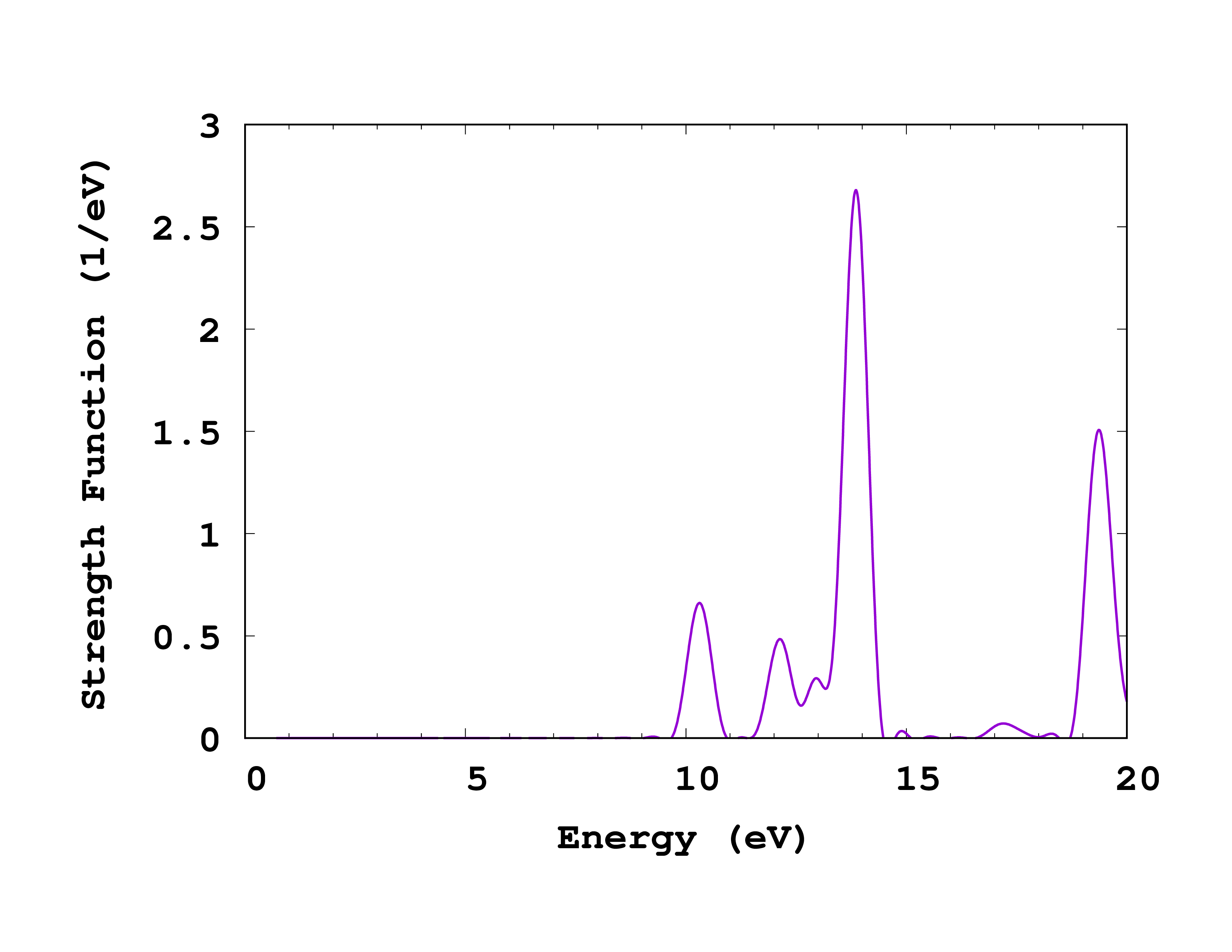
If you now plot the absorption spectrum (column 5 vs 1 in cross_section_vector , but you can use cross_section_tensor for this exercise in case you did propagate in all three directions), you should obtain the plot shown on the right. Of course, you should now try to converge this spectrum with respect to the calculation parameters. In particular:
- Increasing the total propagation time will reduce the width of the peaks. In fact, the width of the peaks in this methods is absolutely artificial, and is inversely proportional to the total propagation time. Do not forget, however, that the area under the peaks has a physical meaning: it is the oscillator strength of the transition.
- A convergence study with respect to the spacing and box size might be necessary. This is covered in the next tutorial.
Some questions to think about:
- What is the equation for the peak width in terms of the propagation time? How does the observed width compare to your expectation?
- What is the highest energy excitation obtainable with the calculation parameters here? Which is the key one controlling the maximum energy?
- Why does the spectrum go below zero? Is this physical? What calculation parameters might change this?