Basic QOCT
If you set CalculationMode = opt_control, you will be attempting to solve
the Quantum Optimal Control Theory (QOCT) equations. This tutorial introduces the basic theoretical concepts of
QOCT, as well as the procedure to perform basic QOCT calculations with Octopus.
If you already know QOCT, you can skip the Theoretical Introduction.
Theoretical Introduction
The QOCT can be formulated in the following way:
We consider a quantum mechanical system, governed in a temporal interval $[0,T]$ by the Hamiltonian $\hat{H}[\varepsilon(t)]$. The Hamiltonian depends parametrically on a “control parameter” $\varepsilon(t)$. In the cases we are concerned with, this is the temporal shape of an external electromagnetic field, typically the temporal shape of a laser pulse. This Hamiltonian drives the system from one specified initial state $\vert\Psi_0\rangle$ to a final state $\vert\Psi(T)\rangle$, according to Schrödinger’s equation:
$i\frac{\rm d}{{\rm d}t}\vert\Psi(t)\rangle = \hat{H}[\varepsilon(t)]\vert\Psi(t)\rangle,.$
We now wish to find the ‘‘optimal’’ control parameter $\varepsilon$ such that it maximizes a given objective, which in general should be expressed as a functional, $J_1[\Psi]$ of the full evolution of the state. This search must be constrained for two reasons: One, the control parameter must be constrained to ‘‘physical’’ values – that is, the laser field cannot acquire unlimitedly large values. Two, the evolution of the state must obviously follow Schrödinger equation.
These considerations are translated into mathematical terms by prescribing the maximization of the following functional:
$J[\Psi,\chi,\varepsilon] = J_1[\Psi] + J_2[\varepsilon] + J_3[\Psi,\chi,\varepsilon]\,.$
-
$J_1[\Psi]$ is the objective functional. In this basic tutorial, we will be concerned with the case in which it depends only on the value of the state at the end of the propagation, $\Psi(T)$. Moreover, the functional is the expectation value of some positive-definite operator $\hat{O}$:
$J_1[\Psi] = \langle\Psi(T)\vert\hat{O}\vert\Psi(T)\rangle\,.$ -
$J_2[\varepsilon]$ should constrain the values of the control parameter. Typically, the idea is to maximize the objective $J_1$ while minimizing the ‘‘fluence’':
$J_2[\varepsilon] = -\alpha\int_0^T {\rm d}t \varepsilon^2(t)\,.$
The constant $\alpha$ is usually called ‘‘penalty’’. -
The maximization of $J_3$ must ensure the verification of Schrödinger’s equation:
$J_3[\Psi,\chi,\varepsilon] = -2 \Im \left[ \int_0^T {\rm d}t\langle\chi(t)\vert i\frac{\rm d}{{\rm d}t} - \hat{H}[\varepsilon(t)] \vert\Psi(t)\rangle \right]$
The auxiliary state $\chi$ plays the role of a Lagrangian multiplier.
In order to obtain the threesome $(\Psi,\chi,\varepsilon)$ that maximizes this functional we must find the solution to the corresponding Euler equation. The functional derivation leads to the QOCT equations:
$i\frac{\rm d}{{\rm d}t}\vert\Psi(t)\rangle = \hat{H}[\varepsilon(t)]\vert\Psi(t)\rangle\,,$
$\vert\Psi(0)\rangle = \vert\Psi_0\rangle\,.$
$i\frac{\rm d}{{\rm d}t}\vert\chi(t)\rangle = \hat{H}^\dagger[\varepsilon(t)]\vert\chi(t)\rangle\,,$
$\vert\chi(T)\rangle = \hat{O}\vert\Psi(T)\rangle\,,$
$\alpha\varepsilon(t) = \Im \left[ \langle\chi(t)\vert \frac{\partial \hat{H}}{\partial \varepsilon}\vert\Psi(t)\rangle\right]\,.$
Population target: scheme of Zhu, Botina and Rabitz
An important case in QOCT is when we want to achieve a large transition probability from a specific initial state into a final target state. That is, the operator $\hat{O}$ is the projection onto one given ‘‘target’’ state, $\Psi_t$:
$J_1[\Psi] = \vert \langle \Psi(T)\vert\Psi_t\rangle \vert^2 $
As observed by Zhu, Botina and Rabitz1, for this case one can use an alternative definition of $J_3$:
$ J_3[\Psi,\chi,\varepsilon] = -2\Im [ \langle\Psi(T)\vert\Psi_t\rangle \int_0^T {\rm d}t \langle\chi(t)\vert i\frac{\rm d}{{\rm d}t}-\hat{H}[\varepsilon(t)]\vert\Psi(t)\rangle ] $
This alternative definition has the virtue of decoupling the equations for $\chi$ and $\Psi$:
$i\frac{\rm d}{{\rm d}t}\vert\Psi(t)\rangle = \hat{H}[\varepsilon(t)]\vert\Psi(t)\rangle\,,$
$\vert\Psi(0)\rangle = \vert\Psi_0\rangle\,.$
$i\frac{\rm d}{{\rm d}t}\vert\chi(t)\rangle = \hat{H}^\dagger[\varepsilon(t)]\vert\chi(t)\rangle\,,$
$\vert\chi(T)\rangle = \vert\Psi_t\rangle\,,$
$\alpha\varepsilon(t) = \Im \left[ \langle\chi(t)\vert \frac{\partial \hat{H}}{\partial \varepsilon}\vert\Psi(t)\rangle\right]\,.$
These are the equation that we are concerned with in the present example.
The asymmetric double well: preparing the states
We are now going to solve the previous equations, for the case of attempting a transition from the ground state of a given system, to the first excited state. The system that we have chosen is a one-dimensional asymmetric double well, characterized by the potential:
$V(x) = \frac{\omega_0^4}{64B}x^4 - \frac{\omega_0^2}{4}x^2 + \beta x^3 $
Let us fix the parameter values to $\omega_0 = B = 1$ and $\beta=\frac{1}{256}$. The ground state of this system may be obtained with Octopus running the following inp file:
 CalculationMode = gs
 Dimensions = 1
 FromScratch = yes
 BoxShape = sphere
 Spacing = 0.1
 Radius = 8.0
 TheoryLevel = independent_particles
 %Species
 "AWD1D" | species_user_defined | potential_formula | "1/64*(x)^4-1/4*(x)^2+1/256*(x)^3" | valence | 1
 %
 %Coordinates
 "AWD1D" | 0
 %
 ExtraStates = 1
 EigensolverTolerance = 1.0e-6
 EigensolverMaxIter = 1000
 Mixing = 1.0
 MixingScheme = linear
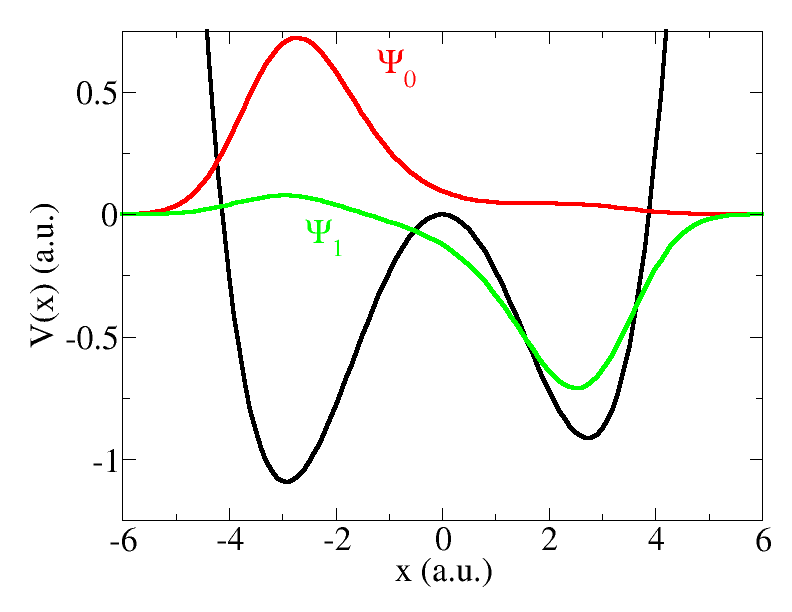
Note that we have set ExtraStates=1 because we want to get the first excited state, in order to be able to do QOCT later (the objective will be the maximum population of this state).
In this way we obtain the first two (single particle) states for this system. It is useful to make a plot with the results, together with the potential. If you do this, you should the curves depicted in Fig. 1. Observe how the ground state is localized in the left well (which is, not surprisingly, deeper), whereas the first excited state is localized in the right well. We are going to attempt to transfer the wavepacket from one side to the other. The energies of these two states are -0.6206 a.u. and -0.4638, respectively.
Note that, in order to plot the functions, you will have to add to the inp file the variables Output and OutputFormat.
Running Octopus in QOCT mode
We now run the code with the following inp file:
 ExperimentalFeatures = yes
 Dimensions = 1
 FromScratch = yes
 CalculationMode = opt_control
 ###################
 # Grid
 ###################
 BoxShape = sphere
 Spacing = 0.1
 Radius = 8.0
 ###################
 # System
 ###################
 %Species
 "ADW1D" | species_user_defined | potential_formula | "1/64*(x)^4-1/4*(x)^2+1/256*(x)^3" | valence | 1
 %
 %Coordinates
 "ADW1D" | 0
 %
 TheoryLevel = independent_particles
 ###################
 # TD RUN Parameters
 ###################
 stime = 100.0
 dt = 0.01
 TDPropagator = aetrs
 TDExponentialMethod = taylor
 TDExponentialOrder = 4
 TDLanczosTol = 5.0e-5
 TDMaxSteps = stime/dt
 TDTimeStep = dt
 ###################
 # OCT parameters
 ###################
 OCTPenalty =1.0
 OCTEps = 1.0e-6
 OCTMaxIter = 50
 OCTInitialState = oct_is_groundstate
 OCTTargetOperator = oct_tg_gstransformation
 %OCTTargetTransformStates
 0 | 1
 %
 OCTScheme = oct_zbr98
 OCTDoubleCheck = yes
 ###################
 # Laser field = Initial guess
 ###################
 ampl = 0.06
 freq = 0.157
 %TDExternalFields
 electric_field | 1 | 0 | 0 | freq | "envelope_function"
 %
 %TDFunctions
 "envelope_function" | tdf_cw | ampl
 %
 ###################
 # Output
 ###################
 Output = wfs
 OutputFormat = axis_x
 TDOutput = laser + td_occup
Let us go through some of the key elements of this inp file:
-
The first part of the file is just a repetition of the basic information already given in the inp file for the ground state calculation: definition of the system through the Species block, specification of the mesh, etc.
-
Each QOCT run consists of a series of backward-forward propagations for both $\Psi$ and $\chi$; the variables in the section “TD Run parameters” specify how those propagations are done. It is especially important to set the total time of the propagation, which fixes the interval $[0,T]$ mentioned above in the QOCT problem definition.
-
The next section (“OCT parameters”) define the particular way in which OCT will be done:
- OCTScheme is the particular OCT algorithm to be used. For this example, we will use the one suggested by Zhu, Botina and Rabitz1. This choice is “oct_zbr98”.
- OCTMaxIter sets a maximum number of iterations for the the ZBR98 algorithm. Each iterations involves a forward and a backward propagation of the wavefunction.
- OCTEps sets a convergence threshold for the iterative scheme. This iterative scheme can be understood as a functional that processes an input control parameter $\varepsilon_i$ and produces an output control parameters $\varepsilon_o$, Upon convergence, input and output should converge and the iterations stopped. This will happen whenever
$D[\varepsilon_i,\varepsilon_o] = \int_0^T \vert \varepsilon_o(t)-\varepsilon_i(t)\vert^2,.$
is smaller than OCTEps. Note that this may never happen; there is no convergence guarantee. - OCTPenalty sets the $\alpha$ penalty parameter described previously.
- OCTInitialState should specify the initial states from which the propagation starts. In most cases this will just be the ground state of the system – this is the case for this example. The value “oct_is_groundstate” means that.
- OCTTargetOperator sets which kind of target operator ($\hat{O}$, with the notation used above) will be used. As mentioned before, for this example we will be using a very common kind of target: the projection onto a target state: $\hat{O}=\vert\Psi_t\rangle\langle\Psi_t\vert$. This is set by doing OCTTargetOperator = oct_tg_gstransformation. This means that the target state is constructed by taking a linear combination of the spin-orbitals that form the ground state. The particular linear combination to be used is set by the block OCTTargetTransformStates.
- OCTTargetTransformStates. This is a block. Each line of the code refers to each of the spin orbitals that form the state the system; in this example we have a one-particle problem, and therefore one single spin-orbital. This spin orbital will be a linear combination of the spin-orbitals calculated in the previous ground-state run; each of the columns will contain the corresponding coefficient. In our case, we calculated two spin-orbitals in the ground state run, therefore we only need two columns. And our target state is simply the first excited state, so the first column (coefficient of the ground state orbital) is zero, and the second column is one.
- OCTDoubleCheck simply asks the code to perform a final propagation with the best field it could find during the QOCT iterative scheme, to check that it is really working as promised.
- The next section (“Laser field = Initial guess”) simply specifies which is the initial laser field to be used as “initial guess”. It is mandatory, since it not only provides with the initial guess for the “control parameter” (which is simply a real function $\varepsilon(t)$ that specifies the temporal shape of the time-dependent external perturbation), but also specifies what kind of external perturbation we are talking about: an electric field with x, y or z polarization, a magnetic field, etc.
- Finally, we would like to do cute plots with our results, so we add an “Output” section. This only applies if we have set OCTDoubleCheck=yes, since the code does not plot anything during the propagations performed in the QOCT iterations. The variables given will permit us to plot the shape of the wavefunction during the propagation, as well as the time-dependent electric field and the projection of the propagating wave function onto the ground state and first excited state.
Even if this is a simple one-dimensional system, the run will take a few minutes because we are doing a lot of propagations. You will see how, at each iteration, some information is printed to standard output, e.g.:
 ****************** Optimal control iteration -   12 ******************
        => J1       =      0.87422
        => J        =      0.54580
        => J2       =     -0.32842
        => Fluence  =      0.32842
        => Penalty  =      1.00000
        => D[e,e']  =     1.66E-04
 **********************************************************************
The meaning of each number should be clear from the notation that we have introduced above. By construction, the algorithm is “monotonously convergent”, meaning that the value of $J$ should increase. This does not guarantee that the final value of $J_1$ will actually approach one, which is our target (full overlap with the first excited state), but we certainly hope so.
At the end of the run it will do a “final propagation with the best field” (usually the one corresponding to the last iteration). For this example, you will get something like:
 *************** Final propagation with the best field ****************
        => J1       =      0.94926
        => J        =      0.61505
        => J2       =     -0.33420
        => Fluence  =      0.33420
 **********************************************************************
So we ‘‘almost’’ achieved a full transfer: $J_1[\Psi]=\vert\langle\Psi(T)\vert\Psi_t\rangle\vert^2 = 0.94926$.
Analysis of the results
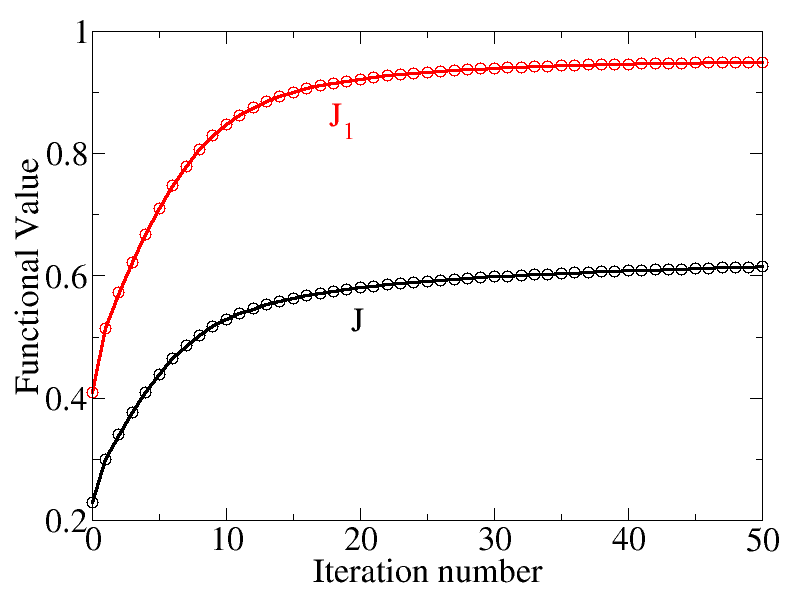
The run will create a directory called opt-control (among others). In it there is a file called convergence that contains the convergence history of the QOCT run, i.e. the values of the relevant functionals at each QOCT iteration. It is useful to make a plot with these values; you can see the result of this in Fig. 2. Observe the monotonous increase of $J$. Also, in this case, the functional $J_1$ (which is, in fact, the one we are really interested in) grows and approaches unity – although the final limit will not be one, but in this case something close to 0.95.
You may want to get the laser pulses used at each iteration, you can do so by setting the variable OCTDumpIntermediate.
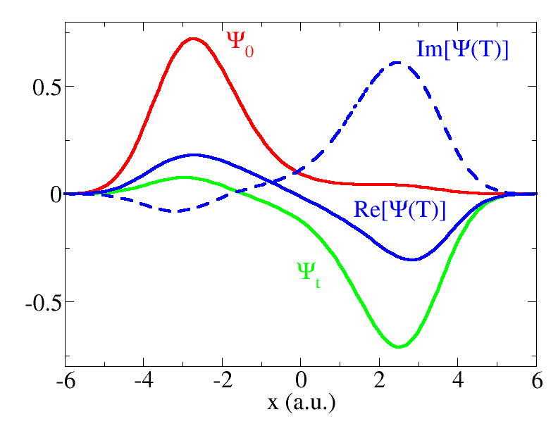
There is also a directory called initial , useful to plot the initial state; a directory called target , that contains the target state; and a directory called final that contains the state at the end of the propagation corresponding to the last QOCT iteration. Fig. 3 is a plot constructed with the information contained in these directories. Note that while the initial and target states have no imaginary part, the final propagated wavefunction is complex, and therefore we have to plot both the real and the imaginary part.
In the directories laser.xxxx you will find a file called cp which contains the control parameter for the corresponding QOCT iteration. Another file, called Fluence informs about the corresponding fluence. The format of file cp is simple: first column is time, second and third column are the real and imaginary part of the control parameter. Since $\varepsilon$ is defined to be real in our formulation, the last column should be null. Finally, the directory laser.bestJ1 will obviously contain the control parameter corresponding to the iteration that produced the best $J_1$.
-
W. Zhu, J. Botina and H. Rabitz, J. Chem. Phys. ‘‘‘108’'’, 1953 (1998) ↩︎