Convergence of the optical spectra
In the previous Optical Spectra from TD we have seen how to obtain the absorption spectrum of a molecule. Here we will perform a convergence study of the spectrum with respect to the grid parameters using again the methane molecule as an example.
Convergence with the spacing
In the Total energy convergence tutorial we found out that the total energy of the methane molecule was converged to within 0.1 eV for a spacing of 0.18 Å and a radius of 3.5 Å. We will therefore use these values as a starting point for our convergence study. Like for the total energy, the only way to check if the absorption spectrum is converged with respect to the spacing is by repeating a series of calculations, with identical input files except for the grid spacing. The main difference in this case is that each calculation for a given spacing requires several steps:
- Ground-state calculation,
- Three time-dependent propagations with perturbations along ‘‘x’’, ‘‘y’’ and ‘‘z’’,
- Calculation of the spectrum using the oct-propagation_spectrum utility.
As we have seen before, the $T_d$ symmetry of methane means that the spectrum is identical for all directions, so in this case we only need to perform the convergence study with a perturbation along the ‘‘x’’ direction.
All these calculations can be done by hand, but we would rather use a script for this boring an repetitive task. We will then need the following two files.
inp
This file is the same as the one used in the previous Optical Spectra from TD:
CalculationMode = td
UnitsOutput = eV_angstrom

Radius = 3.5*angstrom
Spacing = 0.18*angstrom

CH = 1.097*angstrom
%Coordinates
 "C" |           0 |          0 |           0
 "H" |  CH/sqrt(3) | CH/sqrt(3) |  CH/sqrt(3)
 "H" | -CH/sqrt(3) |-CH/sqrt(3) |  CH/sqrt(3)
 "H" |  CH/sqrt(3) |-CH/sqrt(3) | -CH/sqrt(3)
 "H" | -CH/sqrt(3) | CH/sqrt(3) | -CH/sqrt(3)
%

TDPropagator = aetrs
TDTimeStep = 0.0023/eV
TDMaxSteps = 4350  # ~ 10.0/TDTimeStep

TDDeltaStrength = 0.01/angstrom
TDPolarizationDirection = 1
spacing.sh
And this is the bash script:
#!/bin/bash
list="0.26 0.24 0.22 0.20 0.18"
export OCT_PARSE_ENV=1
for Spacing in $list
do
    export OCT_Spacing=$(echo $Spacing*1.8897261328856432 | bc)
    export OCT_CalculationMode=gs
    octopus >& out-gs-$Spacing
    export OCT_CalculationMode=td
    octopus >& out-td-$Spacing
    oct-propagation_spectrum >& out-spec-$Spacing
    mv cross_section_vector cross_section_vector-$Spacing
    rm -rf restart
done
unset OCT_Spacing OCT_CalculationMode
This script performs the three steps mentioned above for a given list of spacings. You will notice that we are not including smaller spacings than 0.18 Å. This is because we know from previous experience that the optical spectrum is well converged for spacings larger than the one required to converge the total energy.
Now run the script typing
source spacing.sh
. This will take some time, so you might want to have a break. Once the script is finished running, we need to compare the spectra for the different spacings. Using your favorite plotting software, e.g.
gnuplot
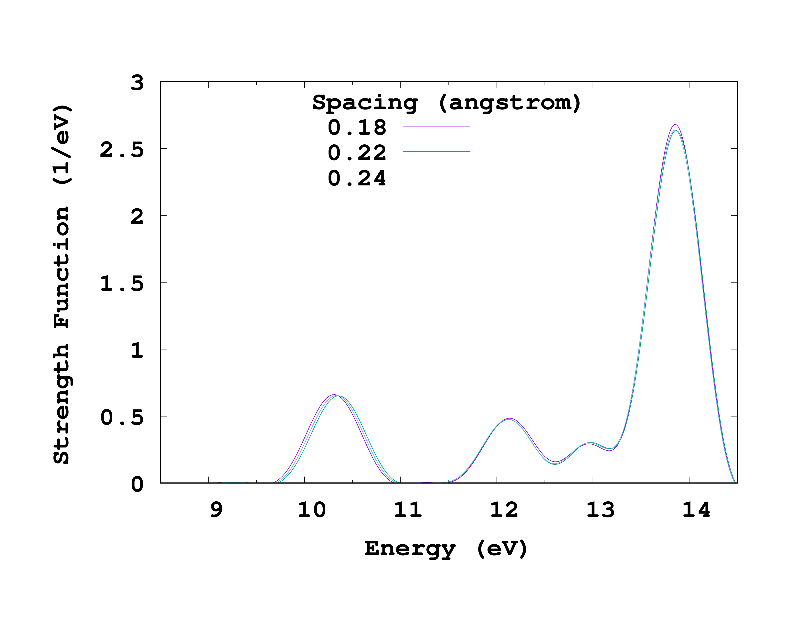
, plot the second column of the cross_section_vector
files vs the first column. You can see on the right how this plot should look like. To make the plot easier to read, we have restricted the energy range and omitted some of the spacings. From the plot it is clear that a spacing of 0.24 Å is sufficient to have the position of the peaks converged to within 0.1 eV.
Convergence with the radius
We will now study how the spectrum changes with the radius. We will proceed as for the spacing, by performing a series of calculations with identical input files except for the radius. For this we will use the two following files.
inp
This file is the same as the prevous one, with the exception of the spacing and the time-step. As we have just seen, a spacing of 0.24 Å is sufficient, which in turns allows us to use a larger time-step.
CalculationMode = td
UnitsOutput = eV_angstrom

Radius = 3.5*angstrom
Spacing = 0.24*angstrom

CH = 1.097*angstrom
%Coordinates
 "C" |           0 |          0 |           0
 "H" |  CH/sqrt(3) | CH/sqrt(3) |  CH/sqrt(3)
 "H" | -CH/sqrt(3) |-CH/sqrt(3) |  CH/sqrt(3)
 "H" |  CH/sqrt(3) |-CH/sqrt(3) | -CH/sqrt(3)
 "H" | -CH/sqrt(3) | CH/sqrt(3) | -CH/sqrt(3)
%

TDPropagator = aetrs
TDTimeStep = 0.004/eV
TDMaxSteps = 2500  # ~ 10.0/TDTimeStep

TDDeltaStrength = 0.01/angstrom
TDPolarizationDirection = 1
radius.sh
And this is the bash script:
#!/bin/bash
list="3.5 4.5 5.5 6.5 7.5"
export OCT_PARSE_ENV=1
for Radius in $list
do
    echo "$Radius"
    export OCT_Radius=$(echo $Radius*1.8897261328856432 | bc)
    export OCT_CalculationMode=gs
    octopus >& out-gs-$Radius
    export OCT_CalculationMode=td
    octopus >& out-td-$Radius
    oct-propagation_spectrum >& out-spec-$Radius
    mv cross_section_vector cross_section_vector-$Radius
    rm -rf restart
done
unset OCT_Radius OCT_CalculationMode
This script works just like the previous one, but changing the radius instead of the spacing. Now run the script ( source radius.sh ) and wait until it is finished.
Now plot the spectra from the cross_section_vector files. You should get something similar to the plot on the right. We see that in this case the changes are quite dramatic. To get the first peak close to 10 eV converged within 0.1 eV a radius of 6.5 Å is necessary. The converged transition energy of 9.2 eV agrees quite well with the experimental value of 9.6 eV and with the TDDFT value of 9.25 eV obtained by other authors.1
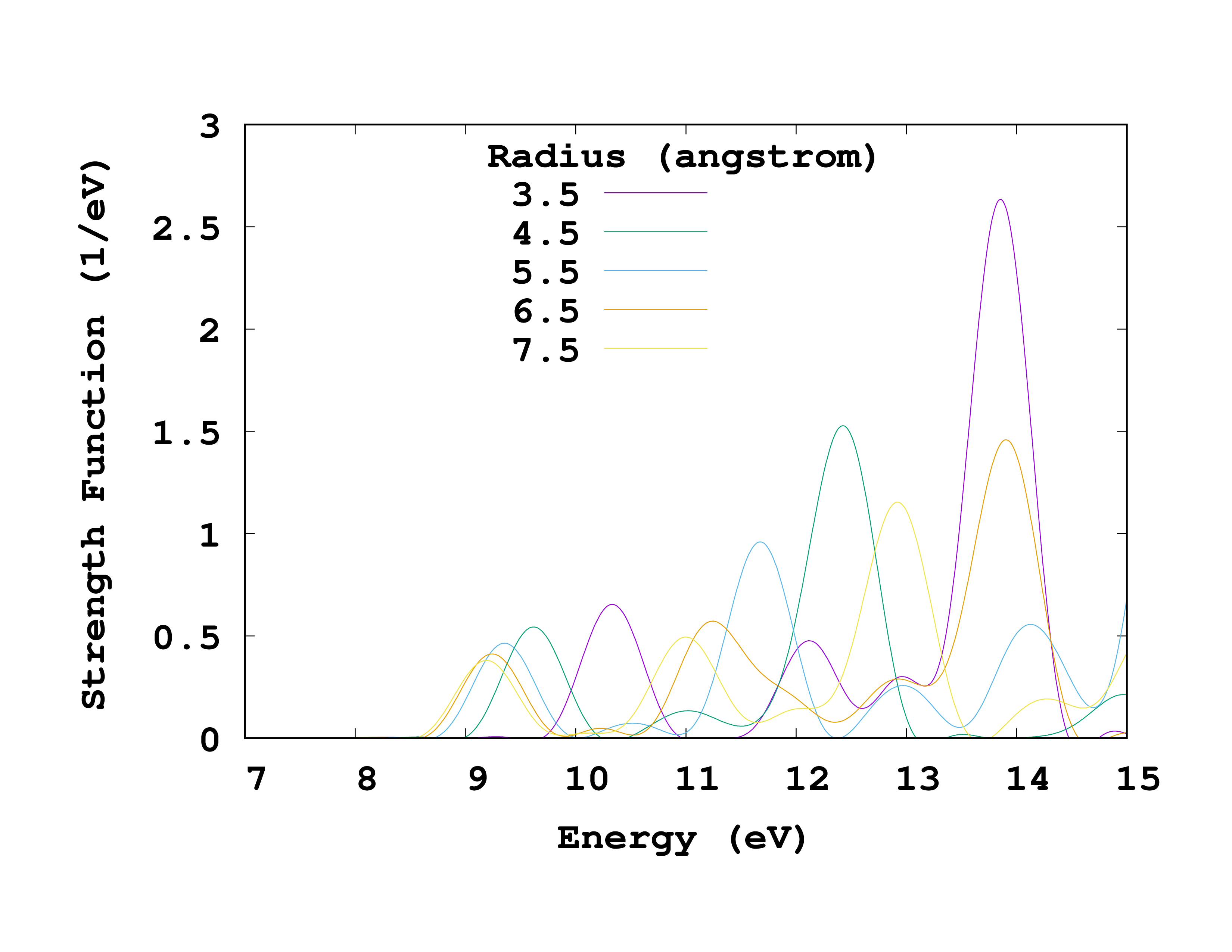
What about the peaks at higher energies? Since we are running in a box with zero boundary conditions, we will also have the box states in the spectrum. The energy of those states will change with the inverse of the size of the box and the corresponding peaks will keep shifting to lower energies. However, as one is usually only interested in bound-bound transitions in the optical or near-ultraviolet regimes, we will stop our convergence study here. As an exercise you might want to converge the next experimentally observed transition. Just keep in mind that calculations with larger boxes might take quite some time to run.
-
N. N. Matsuzawa, A. Ishitani, D. A. Dixon, and T. Uda, Time-Dependent Density Functional Theory Calculations of Photoabsorption Spectra in the Vacuum Ultraviolet Region, J. Phys. Chem. A 105 4953–4962 (2001); ↩︎