Navigation :

Wires and slabs

In this tutorial we will explain how to use the flexibility of the real-space grid to treat systems that are periodic in only one or two dimensions. As examples we will use a Na chain and a hexagonal boron nitride (h-BN) monolayer.

Introduction

In the [Periodic systems](../Periodic systems) tutorial, we saw that the PeriodicDimensions input variable controls the number of dimensions to be considered as periodic. In that tutorial we only considered the case PeriodicDimensions = 3. Let’s now see in detail the different cases:

PeriodicDimensions = 0 (which is the default) gives a finite system calculation, since Dirichlet zero boundary conditions are used at all the borders of the simulation box;
PeriodicDimensions = 1 means that only the ‘‘x’’ axis is periodic, while in all the other directions the system is confined. This value must be used to simulate, for instance, a single infinite wire.
PeriodicDimensions = 2 means that both ‘‘x’’ and ‘‘y’’ axis are periodic, while zero boundary conditions are imposed at the borders crossed by the ‘‘z’’ axis. This value must be used to simulate, for instance, a single infinite slab.
PeriodicDimensions = 3 means that the simulation box is a primitive cell for a fully periodic infinite crystal. Periodic boundary conditions are imposed at all borders.

It is important to understand that performing, for instance, a PeriodicDimensions = 1 calculation in Octopus is not quite the same as performing a PeriodicDimensions = 3 calculation with a large supercell. In the infinite-supercell limit the two approaches reach the same ground state, but this does not hold for the excited states of the system.

Another point worth noting is how the Hartree potential is calculated for periodic systems. In fact the discrete Fourier transform that are used internally in a periodic calculation would always result in a 3D periodic lattice of identical replicas of the simulation box, even if only one or two dimensions are periodic. Fortunately Octopus includes a clever system to exactly truncate the long-range part of the Coulomb interaction, in such a way that we can effectively suppress the interactions between replicas of the system along non-periodic axes ¹ . This is done automatically, since the value of PoissonSolver in a periodic calculation is chosen according to PeriodicDimensions. See also the variable documentation for PoissonSolver.

Atomic positions

An important point when dealing with semi-periodic systems is that the coordinates of the atoms along the aperiodic directions must be centered around 0, as this is the case for isolated systems. For slabs, this means that the atoms of the slab must be centered around z=0. If this is not the case, the calculation will lead to wrong results.

Sodium chain

Let us now calculate some bands for a simple single Na chain (i.e. not a crystal of infinite parallel chains, but just a single infinite chain confined in the other two dimensions).

Ground-state

First we start we the ground-state calculation using the following input file:

 CalculationMode = gs
  UnitsOutput = ev_angstrom
 ExperimentalFeatures = yes
 
 PeriodicDimensions = 1
 
 Spacing = 0.3*angstrom
  
 %Lsize
  1.99932905*angstrom | 5.29*angstrom | 5.29*angstrom
 %
 
 %Coordinates
  "Na" | 0.0 | 0.0 | 0.0
 %
 
 %KPointsGrid
  9 | 1 | 1
 %
 KPointsUseSymmetries = yes

Most of these input variables were already introduced in the [Periodic systems](../Periodic systems) tutorial. Just note that the ‘‘k’'-points are all along the first dimension, as that is the only periodic dimension.

The output should be quite familiar, but the following piece of output confirms that the code is indeed using a cutoff for the calculation of the Hartree potential, as mentioned in the Introduction:


****************************** Hartree *******************************
The chosen Poisson solver is 'fast Fourier transform'
Input: [PoissonFFTKernel = cylindrical]
**********************************************************************

Input: [FFTLibrary = fftw]
Info: FFT grid dimensions       = 13 x 75 x 75
      Total grid size           = 73125 (   0.6 MiB )
      Inefficient FFT grid. A better grid would be: 14 75 75
Info: Poisson Cutoff Radius     =  11.2 A

The cutoff used is a cylindrical cutoff and, by comparing the FFT grid dimensions with the size of the simulation box, we see that the Poisson solver is using a supercell doubled in size in the ‘‘y’’ and ‘‘z’’ directions.

At this point you might want to play around with the number of ‘‘k’'-points until you are sure the calculation is converged.

Band structure

We now modify the input file in the following way:

Band structure for a infinite chain of Sodium atoms, calculated for a single chain (purple lines), and a 3D-periodic crystal of chains in a supercell (green lines).

 CalculationMode = unocc
  UnitsOutput = ev_angstrom
 ExperimentalFeatures = yes
 
 PeriodicDimensions = 1
 
 Spacing = 0.3*angstrom
  
 %Lsize
  1.99932905*angstrom | 5.29*angstrom | 5.29*angstrom
 %
 
 %Coordinates
  "Na" | 0.0 | 0.0 | 0.0
 %
 
 ExtraStates = 6
 ExtraStatesToConverge = 4
 
 %KPointsPath
  14
  0.0 | 0.0 | 0.0
  0.5 | 0.0 | 0.0
 %
 KPointsUseSymmetries = no

and run the code. You might notice the comments on the the LCAO in the output. What’s going on? Why can’t a full initialization with LCAO be done?

You can now plot the band structure using the data from the static/bandstructure file, just like in the [Periodic systems](../Periodic systems) tutorial.

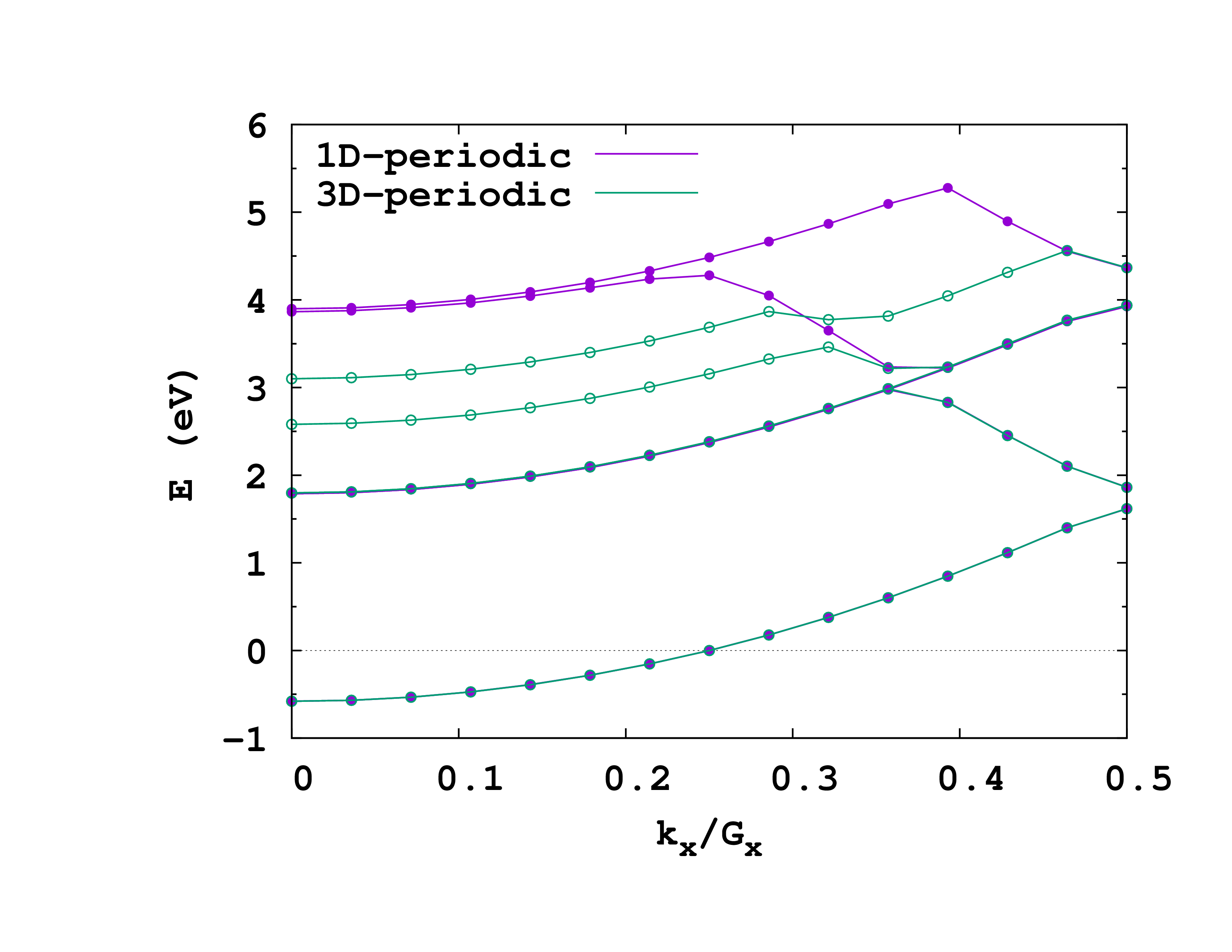
In the introduction we mentioned that performing a calculation with PeriodicDimensions = 1 is not quite the same as performing a PeriodicDimensions= 3 calculation with a large supercell. Lets now check this. Re-run both the ground-state and the unoccupied calculations, but setting PeriodicDimensions = 3 in the above input files. Before doing so, make sure you copy the static/bandstructure file to a different place so that it is not overwritten (better yet, run the new calculations in a different folder). You can see the plot of the two band structures on the right. More comments on this in ref. ¹.

h-BN monolayer

Hexagonal boron nitride (h-BN) is an insulator widely studied which has a similar structure to graphene. Here we will describe how to get the band structure of an h-BN monolayer.

Ground-state calculation

We will start by calculating the ground-state using the following input file:

 CalculationMode = gs
 UnitsOutput = ev_angstrom
 ExperimentalFeatures = yes
 
 PeriodicDimensions = 2
 
 Spacing = 0.20*angstrom
 
 BNlength = 1.445*angstrom
 a = sqrt(3)*BNlength
 L = 40
 %LatticeParameters
  a | a | L
 %
 
 %LatticeVectors
   1.0 | 0.0       | 0.0
  -1/2 | sqrt(3)/2 | 0.0
   0.0 | 0.0       | 1.0
 %
  
 %ReducedCoordinates
  'B' | 0.0 | 0.0 | 0.0
  'N' | 1/3 | 2/3 | 0.0
 % 
 
 PseudopotentialSet=hgh_lda
 
 LCAOStart=lcao_states 
 
 %KPointsGrid
   12   | 12   | 1
 %
 KPointsUseSymmetries = yes

Most of the file should be self-explanatory, but here is a more detailed explanation for some of the choices:

PeriodicDimensions = 2: A layer of h-BN is periodic in the ‘‘x’'-‘‘y’’ directions, but not in the ‘‘z’’ direction, so there are two periodic dimensions.
LatticeParameters: Here we have set the bond length to 1.445 Å. The box size in the ‘‘z’’ direction is ‘‘2 L’’ with ‘‘L’’ large enough to describe a monolayer in the vacuum. Remember that one should always check the convergence of any quantities of interest with the box length value.

If you now run the code, you will notice that the cutoff used for the calculation of the Hartree potential is different than for the Sodium chain, as is to be expected:


****************************** Hartree *******************************
The chosen Poisson solver is 'fast Fourier transform'
Input: [PoissonFFTKernel = planar]
**********************************************************************

Input: [FFTLibrary = fftw]
Info: FFT grid dimensions       = 13 x 13 x 225
      Total grid size           = 38025 (   0.3 MiB )
      Inefficient FFT grid. A better grid would be: 14 14 225
Info: Poisson Cutoff Radius     =  22.5 A

Band Structure

After the ground-state calculation, we will now calculate the band structure. This is the input for the non-self consistent calculation:

 CalculationMode = gs
 UnitsOutput = ev_angstrom
 ExperimentalFeatures = yes
 
 PeriodicDimensions = 2
 
 Spacing = 0.20*angstrom
 
 BNlength = 1.445*angstrom
 a = sqrt(3)*BNlength
 L = 40
 %LatticeParameters
  a | a | L
 %
 
 %LatticeVectors
   1.0 | 0.0       | 0.0
  -1/2 | sqrt(3)/2 | 0.0
   0.0 | 0.0       | 1.0
 %
  
 %ReducedCoordinates
  'B' | 0.0 | 0.0 | 0.0
  'N' | 1/3 | 2/3 | 0.0
 % 
 
 PseudopotentialSet=hgh_lda
 
 LCAOStart=lcao_states 
 
 ExtraStatesToConverge  = 4
 ExtraStates  = 8
 
 %KPointsPath
  12  | 7   | 12   - Number of k point to sample each path
  0.0 | 0.0 | 0.0  - Reduced coordinate of the 'Gamma' k point
  1/3 | 1/3 | 0.0  - Reduced coordinate of the 'K' k point
  1/2 | 0.0 | 0.0  - Reduced coordinate of the 'M' k point
  0.0 | 0.0 | 0.0  - Reduced coordinate of the 'Gamma' k point
 %
 KPointsUseSymmetries = no

Band structure of a monolayer h-BN.

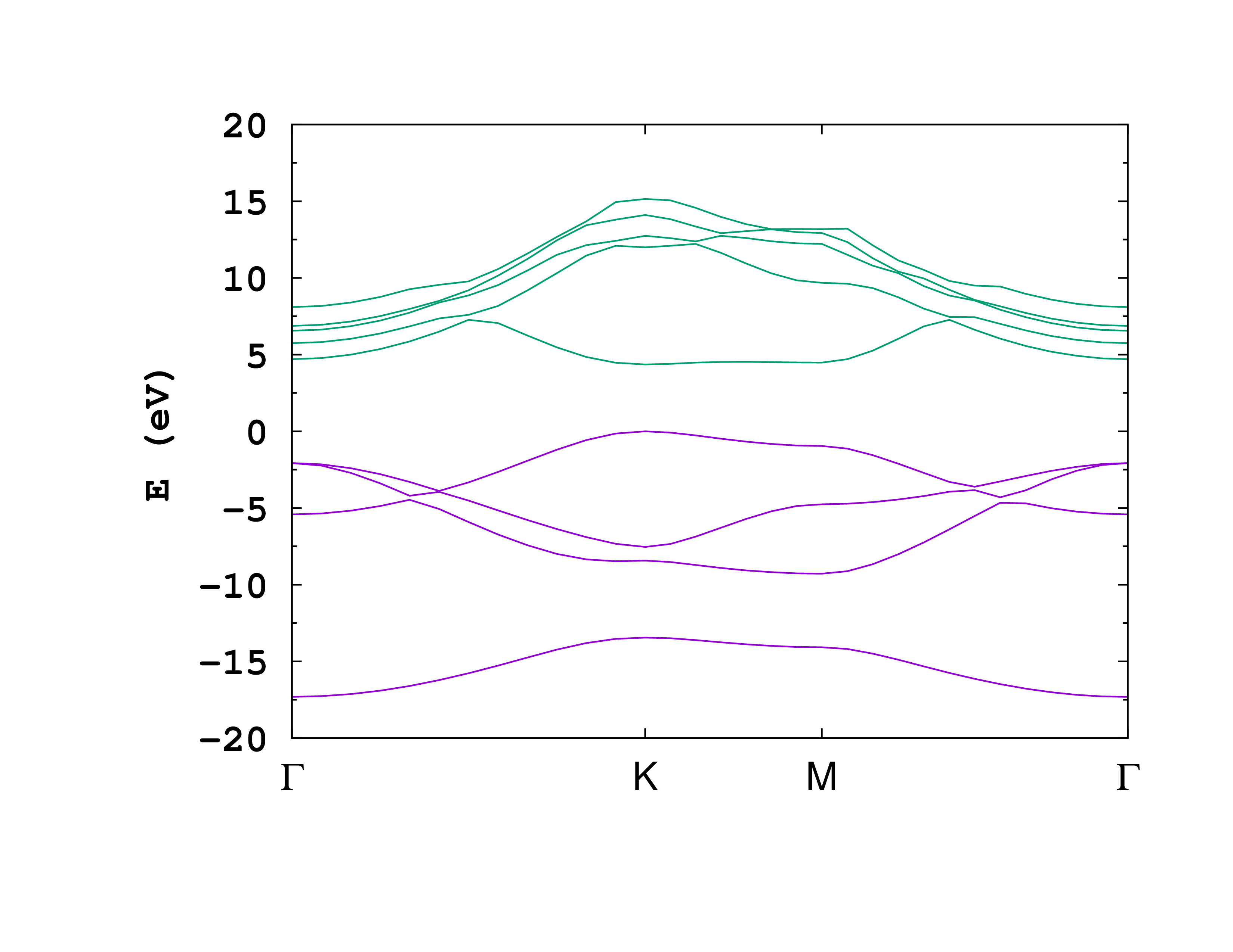
In this case, we chose the following path to calculate the band structure: Gamma-K, K-M, M-Gamma, with a sampling of 12-7-12 ‘‘k’'-points.

On the right is the resulting plot of the occupied bands and the first four unoccupied bands from the static/bandstructure file.

References

C. A. Rozzi, D. Varsano, A. Marini, E. K. U. Gross, and A. Rubio, Exact Coulomb cutoff technique for supercell calculations, Phys. Rev. B 73 205119 (2006); ↩︎