The box shape can be defined in two ways, which are given by the variable
LinearMediumBoxShape: if set to medium_parallelepiped, the
parallelepiped box will be defined by its center, and size in each dimension
through the LinearMediumBoxSize block; if the box shape is
defined as medium_box_file, the box shape will be read from an external OFF
file, defined through the variable LinearMediumBoxFile. To
produce such files, check the Creating geometries tutorial. In either case, the
electromagnetic properties of each medium must be defined in the LinearMediumProperties block, which specifies the relative electric
permittivity, relative magnetic permeability, and the electric and magnetic
conductivities (for lossy media). Finally, the spatial profile assumed to
calculate gradients at the box edges is defined through the LinearMediumEdgeProfile variable, and can be either “edged” or “smooth”
(for linear media shape read from file, it can only be edged).
Linear media are static. Therefore only the propagator
TDSystemPropagator = static
is permitted. By moving the variable TDSystemPropagator into the Maxwell namespace, the default
propagator (which is static) is automatically inherited by the
Medium system and only the propagator for the Maxwell system is explicitly set to exp_mid. As the exp_mid propagator contains two algorithmic steps, it must be clocked
twice as fast as the static propagator and hence the time step
of the medium bust be set to half the Maxwell time step. This is currently a
workaround, and is likely to change in future releases of the code.
To illustrate a laser pulse hitting a linear medium box, in addition to
adding the linear_medium system, we need to switch the Maxwell Hamiltonian
operator from the 3x3 vacuum representation to the 6x6 coupled representation
with the six component Riemann-Silberstein vector that includes also the complex
conjugate Riemann-Silberstein vector.
# ----- Maxwell box variables ---------------------------------------------------------------------

 # free maxwell box limit of 10.0 plus 2.0 for the incident wave boundaries with
 # der_order times dx_mx (here: der_order = 4)

 lsize_mx = 12.0
 dx_mx    = 0.5

 Maxwell.BoxShape = parallelepiped

 %Maxwell.Lsize
  lsize_mx | lsize_mx | lsize_mx
 %

 %Maxwell.Spacing
  dx_mx | dx_mx | dx_mx
 %
For this run, we use the previous incident plane wave propagating only in the
x-direction but place a medium box inside the Simulation box.
# ----- Maxwell field variables -------------------------------------------------------------------

 # laser propagates in x direction

 lambda1 = 10.0
 omega1  = 2 * pi * c / lambda1
 k1_x    = omega1 / c
 E1_z    = 0.05
 pw1     = 10.0
 ps1_x   = - 25.0

 %MaxwellIncidentWaves
   plane_wave_mx_function | 0 | 0 | E1_z | "plane_waves_function_1"
 %

 %MaxwellFunctions
   "plane_waves_function_1" | mxf_cosinoidal_wave | k1_x | 0    | 0 | ps1_x | 0     | 0 | pw1
 %
gnuplot script
set pm3d
set view map
set palette defined (-0.05 "blue", 0 "white", 0.05"red")
set term png size 1000,500

unset surface
unset key

set output 'plot1.png'

set xlabel 'x-direction'
set ylabel 'y-direction'
set cbrange [-0.05:0.05]

set multiplot

set origin 0.025,0
set size 0.45,0.9
set size square
set title 'Electric field E_z (t=0.105328 au)'
sp [-10:10][-10:10] 'Maxwell/output_iter/td.0000050/e_field-z.z=0' u 1:2:3

set origin 0.525,0
set size 0.45,0.9
set size square
set title 'Electric field E_z (t=0.210656 au)'
sp [-10:10][-10:10] 'Maxwell/output_iter/td.0000100/e_field-z.z=0' u 1:2:3

unset multiplot

set output 'plot2.png'

set multiplot

set origin 0.025,0
set size 0.45,0.9
set size square
set title 'Electric field E_z (t=0.263321 au)'
sp [-10:10][-10:10] 'Maxwell/output_iter/td.0000125/e_field-z.z=0' u 1:2:3

set origin 0.525,0
set size 0.45,0.9
set size square
set title 'Electric field E_z (t=0.315985 au)'
sp [-10:10][-10:10] 'Maxwell/output_iter/td.0000150/e_field-z.z=0' u 1:2:3

unset multiplot
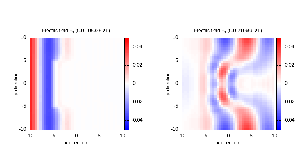
Contour plot of the electric field in z-direction after 50 time steps for
t=0.11 and 100 time steps for t=0.21:
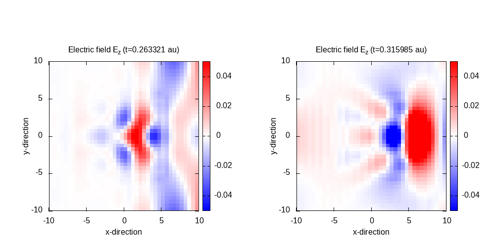
Contour plot of the electric field in z-direction after 125 time steps for
t=0.26 and 150 time steps for t=0.32:
In the last panel, it can be seen that there is a significant amount of
scattered waves which, in large parts, are scattered from the box boundaries.
In the following we will use different boundary conditions, in order to reduce
this spurious scattering.
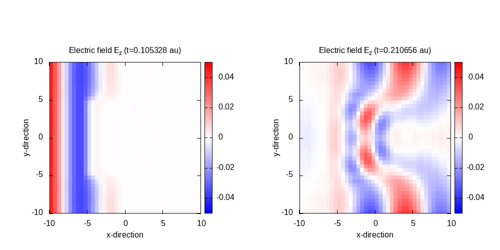
The previous run was without absorbing boundaries, now we switch on the mask
function that damps the field at the boundary by multiplying a scalar mask
function. The MaxwellAbsorbingBoundaries block is updated to
run with mask absorbing. The MaxwellABMaskWidth is set to
five.
As a consequence of the additional region for the absorbing boundary condition,
we have to change the box size to still obtain the same free Maxwell
propagation box. Therefore, the lsize_mx value is now 17.0, which
is the previously used size that includes the incident wave boundary width plus
the absorbing boundary width. For more details, see the information on
simulation boxes
# ----- Maxwell box variables ---------------------------------------------------------------------

 # free maxwell box limit of 10.0 plus 2.0 for the incident wave boundaries with
 # der_order times dx_mx (here: der_order = 4) plus 5.0 for absorbing boundary conditions

 lsize_mx = 17.0
 dx_mx    = 0.5

 Maxwell.BoxShape = parallelepiped

 %Maxwell.Lsize
  lsize_mx | lsize_mx | lsize_mx
 %

 %Maxwell.Spacing
  dx_mx | dx_mx | dx_mx
 %
Contour plot of the electric field in z-direction after 50 time steps for
t=0.11 and 100 time steps for t=0.21:
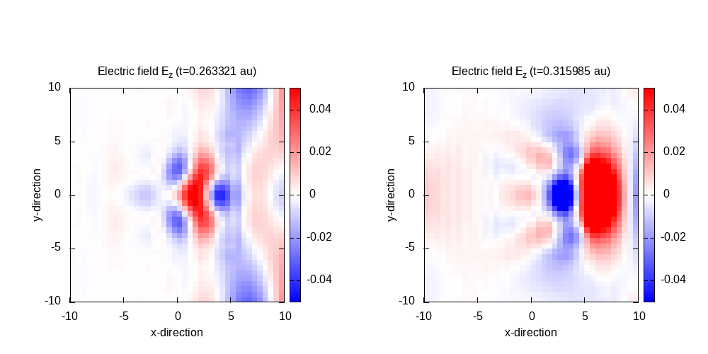
Contour plot of the electric field in z-direction after 125 time steps for
t=0.26 and 150 time steps for t=0.32:
It can be seen that the scattering is slightly reduced, but still noticeable.
The mask absorbing method can be replaced by the more accurate perfectly
matched layer (PML) method. Therefore, the MaxwellAbsorbingBoundaries by the cpml option. The PML
requires some additional parameters to the width for a full definition.