OpenDX
The OpenDX program is no longer supported and the following tutorial should be considered obsolete. We recommend you to use one of the alternatives mentioned in this Visualization.
Input
At this point, the input should be quite familiar to you:
 CalculationMode = gs
 UnitsOutput = eV_Angstrom

 Radius = 5*angstrom
 Spacing = 0.15*angstrom

 Output = wfs + density + elf + potential
 OutputFormat = cube + xcrysden + dx + axis_x + plane_z

 XYZCoordinates = "benzene.xyz"
Coordinates are in this case given in the file benzene.xyz file. This file should look like:
 12
    Geometry of benzene (in Angstrom)
 C  0.000  1.396  0.000
 C  1.209  0.698  0.000
 C  1.209 -0.698  0.000
 C  0.000 -1.396  0.000
 C -1.209 -0.698  0.000
 C -1.209  0.698  0.000
 H  0.000  2.479  0.000
 H  2.147  1.240  0.000
 H  2.147 -1.240  0.000
 H  0.000 -2.479  0.000
 H -2.147 -1.240  0.000
 H -2.147  1.240  0.000
Note that we asked octopus to output the wavefunctions (wfs), the density, the electron localization function (elf) and the Kohn-Sham potential. We ask Octopus to generate this output in several formats, that are requires for the different visualization tools that we mention below. If you want to save some disk space you can just keep the option that corresponds to the program you will use. Take a look at the documentation on variables Output and OutputFormat for the full list of possible quantities to output and formats to visualize them in.
OpenDX
OpenDX is a very powerful, although quite complex, program for the 3D visualization of data. It is completely general-purpose, and uses a visual language to process the data to be plotted. Don’t worry, as you will probably not need to learn this language. We have provided a program (mf.net and mf.cfg ) that you can get from the SHARE/util directory in the Octopus installation (probably it is located in /usr/share/octopus/util ).
Before starting, please make sure you have it installed together with the Chemistry extensions. You may find some instructions [[Releases-OpenDX|here]]. Note that openDX is far from trivial to install and to use. However, the outcomes are really spectacular, so if you are willing to suffer a little at the beginning, we are sure that your efforts will be compensated.
If you run Octopus with this input file, afterward you will find in the static directory several files with the extension .dx . These files contain the wave-functions, the density, etc. in a format that can be understood by [https://www.opendx.org/ Open DX] (you will need the chemistry extensions package installed on top of DX, you can find it in our [[releases]] page).
So, let us start. First copy the files mf.net and mf.cfg to your open directory, and open dx with the command line
> dx
If you followed the instructions given in [[Releases-OpenDX|here]] you should see a window similar to the one shown on the right.
  Image:Tutorial_dx_1.png|Screenshot of the Open DX main menu
  Image:Tutorial_dx_2.png|Main dialog of mf.net
  Image:Tutorial_dx_3.png|Isosurfaces dialog
  Image:Tutorial_dx_4.png|Geometry dialog
Now select ‘''Run Visual Programs…''’, select the mf.net file, and click on ‘''OK''’. This will open the main dialog of our application. You will no longer need the main DX window, so it is perhaps better to minimize it to get it out of the way. Before continuing, go to the menu ‘''Execute > Execute on Change''’, which instructs to open DX to recalculate out plot whenever we make a change in any parameters.
Now, let us choose a file to plot. As you can see, the field File in the mains dialog is NULL. If you click on the three dots next to the field a file selector will open. Just select the file static/density-1.dx and press OK. Now we will instruct open DX to draw a iso-surface. Click on Isosurfaces and a new dialog box will open (to close that dialog box, please click again on Isosurfaces in the main dialog!) In the end you may have lots of windows lying around, so try to be organized. Then click on Show Isosurface 1 - an image should appear with the density of benzene. You can zoom, rotate, etc the picture if you follow the menu ‘''Options > View control…’'' in the menu of the image panel. You can play also around in the isosurfaces dialog with the Isosurface value in order to make the picture more appealing, change the color, the opacity, etc. You can even plot two isosurfaces with different values.
We hope you are not too disappointed with the picture you just plotted. Densities are usually quite boring (even if the Hohenberg-Kohn theorem proves that they know everything)! You can try to plot other quantities like the electronic localization function, the wave-functions, etc, just by choosing the appropriate file in the main dialog. You can try it later: for now we will stick to the “boring density”.
Let us now add a structure. Close the isosurfaces dialog ‘‘‘by clicking again in Isosurfaces in the main dialog box’'’, and open the Geometry dialog. In the File select the file benzene.xyz , and click on Show Geometry. The geometry should appear beneath the isosurface. You can make bonds appear and disappear by using the slide Bonds length, change its colors, etc. in this dialog.
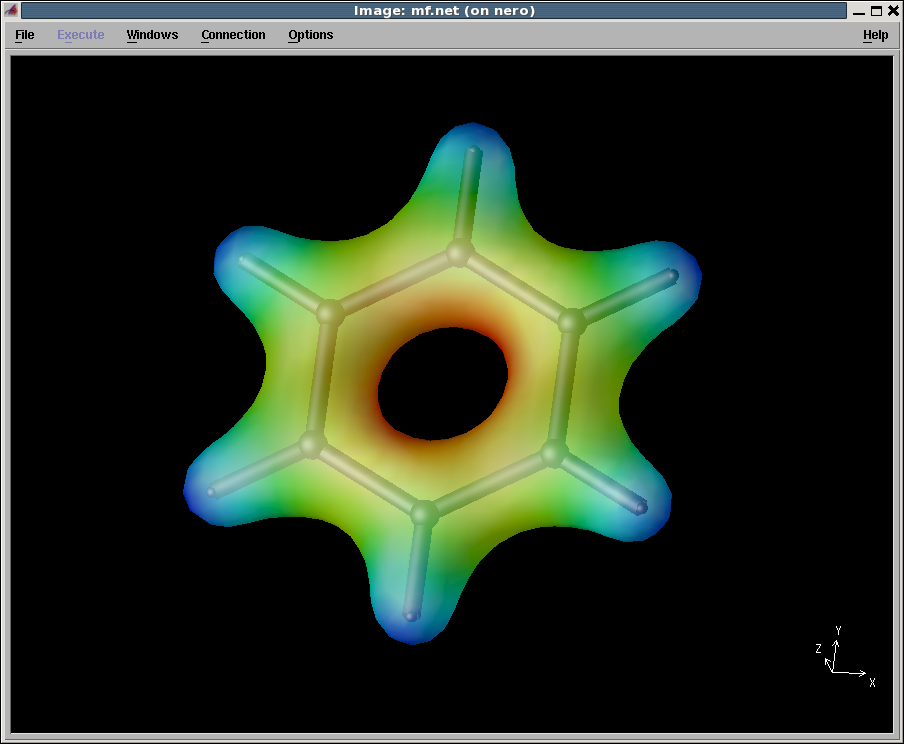
To finish, let us put some “color” in our picture. Close the Geometry dialog (you know how), and open again the isosurfaces dialog. Choose Map isosurface and in the File field choose the file static/vh.dx . There you go, you should have a picture of an isosurface of benzene colored according to the value of the electrostatic potential! Cool, no? If everything went right, you should end with a picture like the one on the right.
As an exercise you can try to plot the wave-functions, etc, make slabs, etc. Play around. As usual some things do not work perfectly, but most of it does!