Open boundaries

This tutorial briefly sketches how to perform calculations with open (or transparent) boundaries in Octopus. Important: Please note that the features described in the following are still subject to changes and further development and certainly not as stable and reliable as required for production runs. Therefore, we very much appreciate feedback and bug reports (or even fixes).

Geometry

Open boundary calculations are only possible for the parallelepiped BoxShape, and only the planes perpendicular to the x-axis are transparent, ‘‘i. e.’’ the transport direction is along the ‘‘x’'-axis, all other boundaries are rigid walls like for the usual finite-system calculations. As the system is open at the “left” and “right” side we have to specify the character of the outside world here. This is done by giving a unit cell of two semi-infinite leads attached to the central or device region, yielding the following geometry (in 2D):

The red area is the device region also constituting the simulation box, ‘‘i. e.’’ the only part in space we treat explicitly in our simulations, which is attached to semi-infinite periodic leads (shown in green). The blue lines indicate the left and right open boundaries.

Overview of the method

Our approach to open-boundary calculations in Octopus generally consists of a three-step procedure:

• A periodic ground-state calculation of the lead unit cell provides the eigenstates of the leads.
• We now scatter these “free” eigenstates in the device region to obtain the ground-state wave functions of the system with broken translational symmetry. This is done by solving a Lippmann-Schwinger equation for the central region. Note: this implies symmetric leads.
• We are now in a position to propagate the ground state of step 2 in time. The system may be perturbed by time-dependent electric and magnetic fields in the central region – just as TDDFT for finite systems – and, additionally, by different left and right time-dependent but spatially constant potentials in the leads (time-dependent bias). The propagation is performed by a modified Crank-Nicolson propagator that explicitly includes the injection of density from the leads and the hopping in and out of the central region by additional source and memory terms. For details, see ¹

Obtaining the ground state

Calculating the ground state for the above geometry requires two runs of Octopus:

• A ground-state calculation of an infinite chain of unit cells of the lead.
• A ground-state calculation of the full system, ‘‘i. e.’’ with the scattering center in place.

We use the multi-dataset capabilities of Octopus to connect the two.

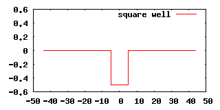
Our first example will calculate the scattering state of an attractive 1D square potential:

We begin with the calculation of the leads which are, in this case, flat and of zero potential, hence, we know that our result should be plane waves. We write the following input file in which we name our periodic dataset lead_ in order to reference it in subsequent calculations:

%CalculationMode
 "lead_"
 gs
%

FromScratch = yes
TheoryLevel = independent_particles

BoxShape = parallelepiped
Dimensions = 1
Spacing = 0.1

%Species
 "flat" | 0 | user_defined | 2.0 | "0"
%


- The lead.
lead_PeriodicDimensions = 1
%lead_Coordinates
 "flat" | 0 | 0 | 0
%

%lead_Lsize
 40*Spacing | 0 | 0
%

%lead_KPoints
 1 | 0.1 | 0 | 0
%

lead_Output = potential
lead_OutputHow = binary

We write out the potential in binary format because it is needed in the next run, where we will scatter the outcome of the periodic run at the square well. The following additions to the the input file will do the job:

%CalculationMode
 "lead_" | "well_"
 gs      | gs
%

<...>

V = 0.5
W = 10
%Species
 "flat" | 0 | user_defined | 2.0 | "0"
 "well" | 0 | user_defined | 2.0 | "V*(-step(x+W/2)+step(x-W/2))"
%

<...>

- The extended system with scattering center.
add_ucells = 2
%well_OpenBoundaries
 lead_dataset     | "lead_"
 lead_restart_dir | "lead_restart"
 lead_static_dir  | "lead_static"
 add_unit_cells   | add_ucells
%

%well_Coordinates
 "well" | 0 | 0 | 0
%

%well_Lsize
 20 | 0 | 0
%

A few points deserve comments:

• The block OpenBoundaries enables the entire open-boundaries machinery. In the block, we have to specify which dataset provided the periodic results. Note that only the lead_ run is periodic by virtue of lead_PeriodicDimensions=1. Furthermore, the algorithm that calculates the ground state of the extended system needs to know where to find the lead potential (line starting with lead_static_dir) and the ground-state wave functions of the lead (line starting with lead_restart_dir).

• The line add_unit_cells is a bit special: it is usually desirable to include the first few unit cells of the lead in the simulation box. To avoid having to put them there by hand Octopus attaches as many unit cells as requested in this line to the simulation box of the dataset with open boundaries, well_ in this case. So keep in mind that this line may significantly increase your grid sizes.

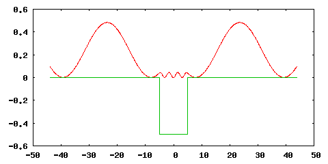
Processing this input file with Octopus gives us the following eigenstate ($|\psi(x)|^2$ is plotted):

Before we turn our attention to a time-propagation, we briefly describe the console output of Octopus related to open boundaries:

• In the Grid section appear two entries. The first one stating that open boundaries are indeed enabled showing the number of unit cells included in the simulation box. The alert reader will note that it says 3 here but 2 in the input file. The reason is that at least one additional unit cell is required by the propagating algorithm into which we will eventually feed our ground-state wave functions. The second one prints how many grid points are in the interface region which is basically determined by the size of the leads’ unit cell.

******************************** Grid ********************************
<...>
Open boundaries in x-direction:
  Additional unit cells left:       3
  Additional unit cells right:      3
  Left lead read from directory:  lead_restart
  Right lead read from directory: lead_restart
<...>
Number of points in left  interface:     80
Number of points in right interface:     80
**********************************************************************

• The following section is also related to open boundaries:

************************ Lead Green functions ************************
 st-  Spin  Lead     Energy
   1   --     L     0.005000
   1   --     R     0.005000
**********************************************************************

The Green’s functions of the leads are required to include the effects of the leads in the Lippmann-Schwinger equation for the simulation region. More information can be found in this [https://www.physik.fu-berlin.de/~lorenzen/physics/transport_nq_yrm08.pdf poster] which was presented at the 5th Nanoquanta Young Researchers Meeting 2008.

Time propagation

We give two small examples for time propagations.

Propagating an eigenstate

As a first time-dependent simulation we simply propagate the eigenstate obtained in the previous section in time without any external influences. We expect that $|\psi(x)|^2$ will not change and that $\psi(x)$ picks up a phase which is shown in this movie:

In order to obtain the input data for the movie we add a third dataset to our input file starting a td calculation:

%CalculationMode
 gs      | gs      | td
 "lead_" | "well_" | "well_"
 1       | 2       | 3
%

Note that this dataset shares label with the ground state run. This enables Octopus to find the correct initial state and avoids the need to repeat the OpenBoundaries block. Apart from the td dataset we only have to give the usual TD parameters: timestep and number of steps in the propagation.

TDMaximumIter = 300
TDTimeStep = 0.5

For completeness, we mention some of Octopus' output related to open boundaries in TD propagations:

************************** Open Boundaries ***************************
Type of memory coefficients:           full
MBytes required for memory term:     59.326
Maximum BiCG iterations:                100
BiCG residual tolerance:            1.0E-12
Included additional terms:              memory source
TD lead potential (L/R):                  0         0
**********************************************************************

This block gives some details about the parameters of the propagation algorithm:

• Both source and memory terms will be included in the simulation (this can be changed by the OpenBoundariesAdditionalTerms variable).
• The memory coefficients are stored as full matrices (by OpenBoundariesMemType) and require 59 MB of main memory.
• The time-dependent potential of the leads is 0.
• The maximum number of iterations solving the Crank-Nicolson system of linear equations is 100 (by OpenBoundariesBiCGMaxiIter) and the tolerance for the iterative solver (OpenBoundariesBiCGTol) is $10^{-12}$.

The calculation of the memory coefficients is accompanied by the oputput

Info: Calculating missing coefficients for memory term of left lead.
[ 52/301]  17%|****                      |     05:06 ETA

and takes very long. Indeed, this is one of the bottlenecks in the algorithm.

Propagation of a Gaussian wavepacket

Our second example is the propagation of a Gaussian-shaped charge distribution in 2D that is initially completely localized in the central region. This calculation is the “standard” test for all implementations of open boundaries. Therefore, it is worth repeating it here. As there are no charges outside the central region we have to disable the source term which is repsonsible for injection of density into our simulation region. Furthermore, the initial state of our time propagation is now given as an entry in the UserDefinedStates block and not as the result of a ground state calculation. Nevertheless, the two ground-state calculations for a completely flat 2D strip have to be performed to initialize certain datastructures.

The part of the input describing the flat 2D strip looks like this:

%CalculationMode
 gs      | gs
 "lead_" | "flat_"
%

FromScratch = yes

TheoryLevel = independent_particles

Dimensions = 2
BoxShape = parallelepiped
Spacing = 0.25

%Species
 "flat" | 0 | user_defined | 2.0 | "0"
%

- The lead.
lead_PeriodicDimensions = 1
%lead_Coordinates
 "flat" | 0 | 0 | 0
%
%lead_Lsize
 4*Spacing | 4 | 0
%
%lead_KPoints
 1 | 0.25 | 0 | 0
%
lead_Output = potential
lead_OutputHow = binary

- The central region.
%flat_OpenBoundaries
 lead_dataset     | "lead_"
 lead_restart_dir | "lead_restart"
 lead_static_dir  | "lead_static"
 add_unit_cells   | 0
%
%flat_Coordinates
 "flat" | 0 | 0 | 0
%
%flat_Lsize
 4 | 4 | 0
%

For the propagation we now override the initial state by giving an explicit formula of a 2D Gaussian wavepacket with initial momentum $(1.75, 1)$

i = {0, 1}
kx = 1.75
ky = 1.0
alpha = 0.5
i = {0, 1}
flat_OnlyUserDefinedInitialStates = yes
%flat_UserDefinedStates
 1 | 1 | 1 | formula | "exp(i*(kx*x + ky*y))*exp(-alpha*r*r)"
%

and add the TD dataset:

%CalculationMode
 gs      | gs      | td
 "lead_" | "flat_" | "flat_"
%

We disable the source term by the line

flat_OpenBoundariesAdditionalTerms = mem_term

The default of OpenBoundariesAdditonalTerms is mem_term + src_term, so solely giving mem_term disables the source term.

Feeding the input into Octopus and generating a movie of $|\psi(x, y, t)|^2$ gives

Since the wavepacket has an initial momentum in the $x$- as well as in $y$-directions, the open boundary at the right and the rigid wall at the back are easily recognized.

References