Polarizable Continuum Model (PCM)
Carlo: How about splitting this tutorial in two parts, so it better fits the categorization or the other tutorials? I propose part 1: "Solvation energy of a molecule in solution within the Polarizable Continuum Model", and part 2: "Time propagation in a solvent within the Polarizable Continuum Model". I have already modified the intros, but I haven't split the page yet, so that Gabriel can finish it first
Solvation energy of a molecule in solution within the Polarizable Continuum Model
In this tutorial we show how calculate the solvation energy of the Hydrogen Fluoride molecule in water solution by setting up a ground state calculation using the Polarizable Continnum Model (PCM).
At the time being PCM is only implemented for TheoryLevel = DFT.
Input
The required input keywords to activate a gs PCM run are PCMCalculation and PCMStaticEpsilon.
PCMCalculation just enables the PCM part of the calculation. PCMStaticEpsilon contains the value of the relative static dielectric constant of the solvent medium (in this particular example water with $\epsilon = 78.39$).
The corresponding minimal input for the ground state calculation in solution is
 CalculationMode = gs
 UnitsOutput = eV_Angstrom

 Radius = 3.5*angstrom
 Spacing = 0.18*angstrom

 PseudopotentialSet = hgh_lda

 FH = 0.917*angstrom
 %Coordinates
  "H" |   0 | 0 | 0
  "F" |  FH | 0 | 0
 %

 PCMCalculation = yes
 PCMStaticEpsilon = 78.39
Warnings
- Please note that the latter input example is intended to make you familiar with the running of Octopus for PCM calculations, it does not provide any benchmark for HF molecule.
- Actually, the geometry might not be optimal and the gs energy might not be converged with respect to the Radius and Spacing variables. A new convergence analysis w.r.t. Radius and Spacing (independent of the one in vacuo) is in principle due when PCM is activated.
- Geometry optimization for solvated molecules within Octopus is still under development; it might work properly only when there are minor adjustments in the geometry when passing from vacuuum to the solvent.
- The selection of the PseudopotentialSet and the implicit choice of LDA xc functional for this particular example is arbitrary.
Output
The main output from such a gs PCM calculation is the solvation energy of the system, which can be extracted from the file
- static/info
The actual info file produced from a calculation with the previous output contains the following energetic contributions:
 Energy [eV]:
       Total       =      -680.55034366
       Free        =      -680.55034366
       -----------
       Ion-ion     =       109.92094773
       Eigenvalues =      -120.75757382
       Hartree     =       708.30289945
       Int[n*v_xc] =      -176.84277019
       Exchange    =      -121.31897823
       Correlation =       -13.43829837
       vanderWaals =         0.00000000
       Delta XC    =         0.00000000
       Entropy     =         0.00000000
       -TS         =        -0.00000000
       E_e-solvent =         1.44141920
       E_n-solvent =        -2.34199070
       E_M-solvent =        -0.90057151
       Kinetic     =       556.30947697
       External    =     -1919.42310315
       Non-local   =        42.69395221
E_M-solvent is the solvation energy, which is in turn split in a term due to electrons and another one due to the nuclei, E_e-solvent and E_n-solvent, respectively.
Carlo: add the first few lines of each output file
When we perform the calculation of HF in water using the previous input, a new folder called pcm is created inside the working directory where input file lies. This pcm folder contains the following files:
- cavity_mol.xyz - useful way to visualize the molecule inside the cavity tessellation. The cavity is plotted as a collection of fictitious Hydrogen atoms. Checking up this file is good to be sure that the molecule fits well inside the cavity and that the tessellation doesn’t contain artifacts.
The first lines of the files are:
    62

   H        1.46477445     1.44399256    -0.00000000
   H        1.08627161     1.44399256     0.52096446
   H        0.47384116     1.44399256     0.32197374
- pcm_info.out - a summary of gs PCM calculation containing information on the tessellation and a table of PCM energetic contributions and total polarization charges due electrons and nuclei for all iterations of the SCF cycle. The PCM energetic contributions are split into the interaction energy of: 1) electrons and polarization charges due to electrons Eee, 2) electrons and polarization charges due to nuclei Een, 3) nuclei and polarization charges due to nuclei Enn, and finally, 4) nuclei and polarization charges due to electrons.
Below, an example of the file:
# Configuration: Molecule + Solvent
###################################
# Epsilon(Solvent) =       78.390
#
# Number of interlocking spheres =    1
#
# SPHERE   ELEMENT               CENTER  (X,Y,Z) (A)                    RADIUS (A)
# ------   -------    -------------------------------------------       ----------
#    1       F        0.91700000      0.00000000      0.00000000        1.54440000
#
# Number of tesserae / sphere = 60
#
#
# Total number of tesserae =   60
# Cavity surface area (A^2) =    29.972947
# Cavity volume (A^3) =    15.430073
#
#
#    iter              E_ee                     E_en                     E_nn                     E_ne                     E_M-solv                 Q_pol                    deltaQ^e                 Q_pol                    deltaQ^n
       1            -293.25112588             294.71995750            -296.89466500             294.71995750              -0.70587588              -7.87251916              -0.02542700               7.89664876              -0.00129741
       2            -293.13633571             294.54433718            -296.89466500             294.54433718              -0.94232634              -7.87358521              -0.02436096               7.89664876              -0.00129741
       3            -293.08877935             294.51502795            -296.89466500             294.51502795              -0.95338845              -7.87305159              -0.02489458               7.89664876              -0.00129741
-
pcm_matrix.out - the PCM response matrix. It is printed for advanced debug and specially to check against GAMESS PCM matrix in the same conditions (same solvent dielectric constant, same geometry of the cavity).
-
ASC_e.dat - polarization charges due to the electrons.
-
ASC_n.dat - polarization charges due to the nuclei.
-
ASC_sol.dat - polarization charges due to the full molecule.
Carlo: a word of warning about the signs of these charges here
The format of the polarization charge file is:
cavity position x | cavity position y | cavity position z | polarization charge | label
where | indicates column separation (actually, replace by spaces in the ASC_*.dat files).
Exercises
-
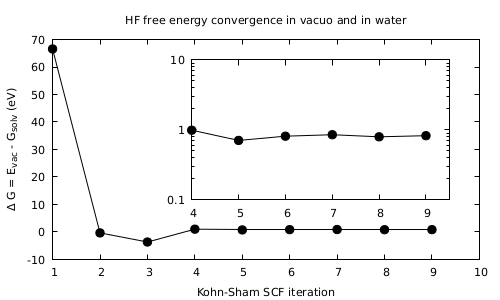
Look first at the convergence of the total energy of the system.
It should look like in the Figure. What it is most important to notice is the fact that there is a stabilization of the system in solvent with respect to the ‘‘in vacuo’’ case. Find the final value and sign of the energy difference between the both cases obtained upon convergence.Carlo: clarify if you mean the energy of the molecule or the solvation energy, and make the figure accordingly
Carlo: Please rename to something meaningful such as PCM_gs_convergence.png and make the figure larger. Mediawiki will thumbnail it automatically. Also I am not sure if the inset is useful. Maybe suggest plotting in log scale as an exercise
-
Another important check is to ascertain whether Gauss’ theorem is fulfilled for the total polarization charges, i.e., if $Q_{pol}=-(\epsilon-1)/\epsilon \times Q_M$ is valid or not, where $Q_M$ is the nominal charge of the molecule. If the latter fails, by setting PCMRenormCharges = yes and manipulating PCMQtotTol Gauss’ theorem is recovered at each SCF iteration (or time-step).
Advanced settings
- The cavity can be improved/refined in several ways.
- You can increase the number of points in the cavity by changing the default value of the variable PCMTessSubdivider from 1 to 4. In practice, the tessellation of each sphere centered at each atomic position (but Hydrogen’s) from 60 to 240 points. Check the convergence and the final value of the total energy with respect to different tessellations.
- You can also relax the constrain on the minimum distance PCMTessMinDistance (=0.1 A by default) between tesserae so as to obtain a more smooth cavity. This might be useful when the geometry of the molecule is complicated. Check if and how the total energy changes.
- You can construct the molecular cavity by putting spheres also in Hydrogen, i.e., by setting PCMSpheresOnH = yes.
- You can change the radius of the spheres used to build up the cavity by manipulating PCMRadiusScaling.
- Moreover, by using PCMCavity = ‘full path to cavity file’ keyword the cavity geometry can be read from a file (instead of being generated inside Octopus, which is the default).
Time propagation in a solvent within the Polarizable Continuum Model
In this tutorial we show how perform a time propagation of the Methene molecule in a solvent by setting up a time-dependent calculation and using the Time-dependent Polarizable Continnum Model (TD-PCM)
As in the case of gas-phase calculations, you should perform always the gs calculation before the td one. At the time being PCM is only implemented for TheoryLevel = DFT.
Carlo: I put the different methods into different sections. Used the same naming as in the octopus paper. Pleas add and comment inputs and outputs.
There are several ways to set up a PCM td calculation in Octopus, corresponding to different kinds of approximation for the coupled evolution of the solute-solvent system.
Equilibrium TD-PCM
The first and most elementary approximation would be to consider an evolution where the solvent is able to instantaneously equilibrate with the solute density fluctuations. Formally within PCM, this means that the dielectric function is constant and equal to its static (zero-frequency) value for all frequencies $\epsilon(\omega)=\epsilon_0$. In practice, this approximation requires minimal changes to the gs input file: just replacing gs by td in the CalculationMode leaving the other PCM related variables unchanged. <span style=“color: red>Carlo: Gabriel, please check that this is corresponds with what you mean
Input
 CalculationMode = td
 UnitsOutput = eV_Angstrom

 Radius = 3.5*angstrom
 Spacing = 0.18*angstrom

 PseudopotentialSet = hgh_lda

 FH = 0.917*angstrom
 %Coordinates
  "H" |   0 | 0 | 0
  "F" |  FH | 0 | 0
 %

 PCMCalculation = yes
 PCMStaticEpsilon = 78.39
Output
Inertial TD-PCM
The first nonequilibrium approximation is to consider that there are fast and slow degrees of freedom of the solvent, of which only the former are able to equilibrate in real time with the solute. The slow degrees of freedom of the solvent that are frozen in time, in equilibrium with the initial (gs) state of the propagation. Formally, it means to consider two dielectric functions for the zero-frequency and high-frequency regime (namely, static and dynamic dielectric constants). In practice, this approximation is finally activated by setting extra input keywords, i.e., PCMTDLevel = neq and PCMDynamicEpsilon, the latter to the dynamic dielectric constant value.
Input
Output
Equation of motion PCM
Finally, in the last –and most accurate– nonequilibrium approximation there is an equation of motion for the evolution of the solvent polarization charges, rendering it history-dependent. Formally, this requires to use a specific model for the frequency-dependence for the dielectric function.