Band structure unfolding
In this tutorial, we look at how to perform a band-structure unfolding using Octopus. This calculation is done in several steps and each one is described below.
Supercell ground-state
The first thing to do is to compute the ground state of a supercell. In this example we will use bulk silicon. The input file is similar to the one used in the Getting started with periodic systems tutorial, but in the present case we will use a supercell composed of 8 atoms. Here is the corresponding input file:
CalculationMode = gs

PeriodicDimensions = 3

Spacing = 0.5

a = 10.18
%LatticeParameters
 a | a  | a
90 | 90 |90
%

%ReducedCoordinates
 "Si" | 0.0         | 0.0       | 0.0
 "Si" |   1/2       | 1/2       | 0.0
 "Si" |   1/2       | 0.0       | 1/2
 "Si" |   0.0       | 1/2       | 1/2
 "Si" |   1/4       | 1/4       | 1/4
 "Si" |   1/4 + 1/2 | 1/4 + 1/2 | 1/4
 "Si" |   1/4 + 1/2 | 1/4       | 1/4 + 1/2
 "Si" |   1/4       | 1/4 + 1/2 | 1/4 + 1/2
%

nk = 4
%KPointsGrid
  nk |  nk |  nk
%
KPointsUseSymmetries = yes

Eigensolver = chebyshev_filter
ExtraStates = 2
All these variables should be familiar from other tutorials. Now run Octopus using this input file to obtain the ground-state of the supercell.
Unfolding setup
After obtaining the ground state of the supercell, we now define the primitive cell on which we want to unfold our supercell and the specific ‘‘k’’-points path that we are interested in. To do this, we take the previous input file and add some new lines:
ExperimentalFeatures = yes
UnfoldMode = unfold_setup
%UnfoldLatticeParameters
  a | a | a
%
%UnfoldLatticeVectors
 0.  | 0.5 | 0.5
 0.5 | 0.  | 0.5
 0.5 | 0.5 | 0.0
%
%UnfoldKPointsPath
 4 | 4 | 8
 0.5 | 0.0 | 0.0 # L point
 0.0 | 0.0 | 0.0 # Gamma point
 0.0 | 0.5 | 0.5 # X point
 1.0 | 1.0 | 1.0 # Another Gamma point
%
Lets see more in detail the input variables that were added:
-
UnfoldMode = unfold_setup: this variable instructs the utility oct-unfold in which mode we are running. As a first step, we are running in the unfold_setup mode, which generates some files that will be necessary for the next steps.
-
UnfoldLatticeParameters specifies the lattice parameters of the primitive cell. This variable is similar to LatticeParameters.
-
UnfoldLatticeVectors specifies the lattice vectors of the primitive cell. This variable is similar to LatticeVectors.
-
UnfoldKPointsPath specifies the ‘‘k’’-points path. The coordinates are indicated as reduced coordinates of the primitive lattice. This variable is similar to KPointsPath.
Now run the oct-unfold utility. You will obtain two files. The first one (unfold_kpt.dat ) contains the list of ‘‘k’’-points of the specified ‘‘k’’-point path, but expressed in reduced coordinates of the supercell. These are the ‘‘k’’-points for which we need to evaluate the wavefunctions of the supercell. The second file (unfold_gvec.dat ) contains the list of reciprocal lattice vectors that relate the ‘‘k’’-points of the primitive cell to the one in the supercell.
Obtaining the wavefunctions
In order to perform the unfolding, we need the wavefunctions in the supercell at specific k-points. These points are described in the unfold_kpt.dat file that we obtained in the previous step. To get the wavefunctions, we need to run a non self-consistent calculation. Here is the corresponding input file:
CalculationMode = unocc

PeriodicDimensions = 3

Spacing = 0.5

a = 10.18
%LatticeParameters
 a | a  | a
90 | 90 |90
%

%ReducedCoordinates
 "Si" | 0.0         | 0.0       | 0.0
 "Si" |   1/2       | 1/2       | 0.0
 "Si" |   1/2       | 0.0       | 1/2
 "Si" |   0.0       | 1/2       | 1/2
 "Si" |   1/4       | 1/4       | 1/4
 "Si" |   1/4 + 1/2 | 1/4 + 1/2 | 1/4
 "Si" |   1/4 + 1/2 | 1/4       | 1/4 + 1/2
 "Si" |   1/4       | 1/4 + 1/2 | 1/4 + 1/2
%

ExperimentalFeatures = yes
UnfoldMode = unfold_setup
%UnfoldLatticeParameters
  a | a | a
%
%UnfoldLatticeVectors
 0.  | 0.5 | 0.5
 0.5 | 0.  | 0.5
 0.5 | 0.5 | 0.0
%
%UnfoldKPointsPath
 4 | 4 | 8
 0.5 | 0.0 | 0.0 # L point
 0.0 | 0.0 | 0.0 # Gamma point
 0.0 | 0.5 | 0.5 # X point
 1.0 | 1.0 | 1.0 # Another Gamma point
%

include unfold_kpt.dat

Eigensolver = chebyshev_filter

ExtraStates = 8
ExtraStatesToConverge = 4
In this input file we have changed the calculation mode (CalculationMode = unocc) and replaced all the ‘‘k’’-points related variables (%KPointsGrid, %KPointsPath, and %KPoints) by the line:
include unfold_kpt.dat
When doing a normal band structure calculation one normally also wants to have some extra states, therefore we have used the ExtraStates and ExtraStatesToConverge variables, as explained in the Getting started with periodic systems tutorial. In this particular case, we are requesting to converge 4 unoccupied states, which all correspond to the first valence band in the folded primitive cell, as the supercell is 4 times larger than the initial cell.
Now run Octopus on this input file.
Note that after you have performed this step, you won’t be able to start a time-dependent calculation from this folder. Indeed, the original ground-state wavefunctions will be replaced by the ones from this last calculation, which are incompatible. Therefore it might be a good idea to create a backup of the restart information before performing this step.
Alternatively, you can continue in a different directory. Instead of copying the restart information to the new folder, you can use the input variable RestartOptions to specify explicitely from which directory the restart files are to be read.
Unfolding
Now that we have computed the states for the required ‘‘k’’-points, we can finally compute the spectral function for each of the ‘‘k’’-points of the specified ‘‘k’’-point path. This is done by changing unfolding mode to be UnfoldMode = unfold_run, so the final input file should look like this:
CalculationMode = unocc

PeriodicDimensions = 3

Spacing = 0.5

a = 10.18
%LatticeParameters
 a | a  | a
90 | 90 |90
%

%ReducedCoordinates
 "Si" | 0.0         | 0.0       | 0.0
 "Si" |   1/2       | 1/2       | 0.0
 "Si" |   1/2       | 0.0       | 1/2
 "Si" |   0.0       | 1/2       | 1/2
 "Si" |   1/4       | 1/4       | 1/4
 "Si" |   1/4 + 1/2 | 1/4 + 1/2 | 1/4
 "Si" |   1/4 + 1/2 | 1/4       | 1/4 + 1/2
 "Si" |   1/4       | 1/4 + 1/2 | 1/4 + 1/2
%

ExperimentalFeatures = yes
UnfoldMode = unfold_run
%UnfoldLatticeParameters
  a | a | a
%
%UnfoldLatticeVectors
 0.  | 0.5 | 0.5
 0.5 | 0.  | 0.5
 0.5 | 0.5 | 0.0
%
%UnfoldKPointsPath
 4 | 4 | 8
 0.5 | 0.0 | 0.0 # L point
 0.0 | 0.0 | 0.0 # Gamma point
 0.0 | 0.5 | 0.5 # X point
 1.0 | 1.0 | 1.0 # Another Gamma point
%

include unfold_kpt.dat

ExtraStates = 6
ExtraStatesToConverge = 4
This will produce the spectral function for the full path (static/ake.dat ) and for each individual points of the path (static/ake_XXX.dat ). The content of the static/ake.dat file should look like this:
#Energy Ak(E)
#Number of points in energy window  1020
 0.000000000000E+00 -2.943437224994E-01  9.234773207848E-02
 0.000000000000E+00 -2.937234225979E-01  9.336366120417E-02
 0.000000000000E+00 -2.931031226963E-01  9.439839874075E-02
 0.000000000000E+00 -2.924828227948E-01  9.545243285977E-02
 0.000000000000E+00 -2.918625228932E-01  9.652626797336E-02
 0.000000000000E+00 -2.912422229917E-01  9.762042539237E-02
 0.000000000000E+00 -2.906219230901E-01  9.873544401596E-02
 0.000000000000E+00 -2.900016231886E-01  9.987188105445E-02
 0.000000000000E+00 -2.893813232870E-01  1.010303127871E-01
 0.000000000000E+00 -2.887610233855E-01  1.022113353570E-01
 0.000000000000E+00 -2.881407234839E-01  1.034155656048E-01
 0.000000000000E+00 -2.875204235824E-01  1.046436419438E-01
 0.000000000000E+00 -2.869001236808E-01  1.058962252792E-01
...
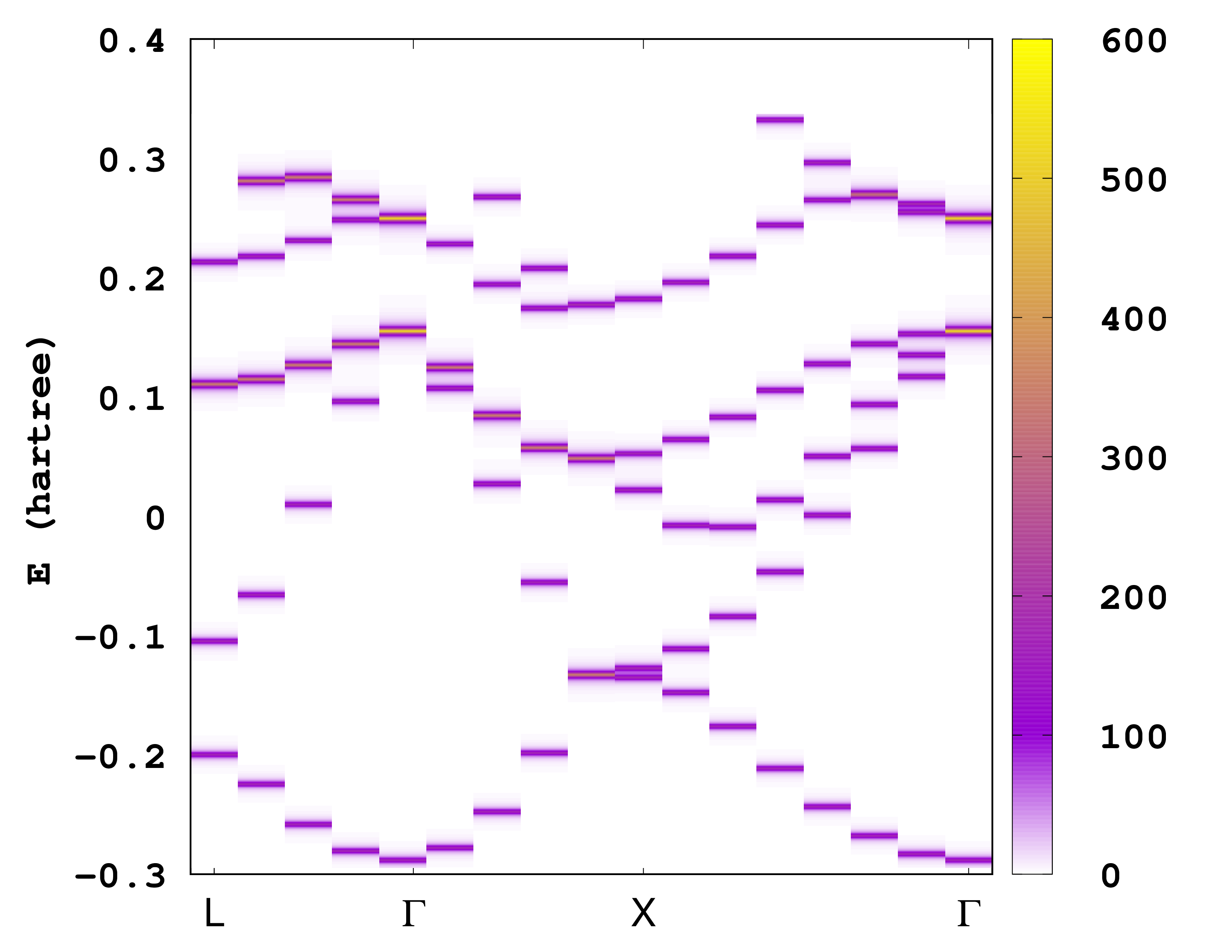
The first column is the coordinate along the ‘‘k’’-point path, the second column is the energy eigenvalue and the last column is the spectral function. There are several ways to plot the information contained in this file. One possibility is to plot it as a heat map. For example, if you are using gnuplot, you can try the following command:
plot 'static/ake.dat' u 1:2:3 w image
The unfolded bandstructure of silicon is shown below. How does it compare to the bandstructure compute in the Getting started with periodic systems?
Note that it is possible to change the energy range and the energy resolution for the unfolded band structure. This is done by specifying the variables UnfoldMinEnergy, UnfoldMaxEnergy, and UnfoldEnergyStep. It is also important to note here that the code needs to read all the unoccupied wavefunctions and therefore might need a large amount of memory, so make sure enough memory is available.