Total energy convergence
In this tutorial we will show how to converge a quantity of interest (the total energy) with respect to the parameters that define the real-space grid. For this we will use two examples, the Nitrogen atom from the Basic input options tutorial, and a methane molecule.
Nitrogen atom: finding a good spacing
The key parameter of a real-space calculation is the spacing between the points of the mesh. The default option in Octopus is to use a Cartesian grid. This is a regular grid where the spacing along each Cartesian direction is the same. The first step in any calculation should then be making sure that this spacing is good enough for our purposes. This should be done through a convergence study, very similar to the ones performed in plane-wave calculations.
The needed spacing essentially depends on the pseudopotentials that are being used. The idea is to repeat a series of ground-state calculations, with identical input files except for the grid spacing. There are many different ways of doing it, the simplest one being to change the input file by hand and run Octopus each time. Another option is to use a little bash script like the one bellow.
As a first example, we will use the Nitrogen atom from the previous tutorial, so make sure you have the corresponding inp
and N.xyz
files in your working directory. Next, create a file called spacing.sh with the following content:
#!/bin/bash
echo "#Sp    Energy        s_eigen   p_eigen" > spacing.dat
list="0.26 0.24 0.22 0.20 0.18 0.16 0.14"
export OCT_PARSE_ENV=1
for Spacing in $list
do
    export OCT_Spacing=$(echo $Spacing*1.8897261328856432 | bc)
    echo $Spacing
    octopus >& out-$Spacing
    energy=`grep Total static/info  | head -1 | cut -d "=" -f 2`
    seigen=`grep  "1   --" static/info | head -1 |  awk '{print $3}'`
    peigen=`grep  "2   --" static/info | head -1 |  awk '{print $3}'`
    echo $Spacing $energy $seigen $peigen >> spacing.dat
    rm -rf restart
done
unset OCT_Spacing
What this script does is quite simple: it runs Octopus for a list of spacings (0.26, 0.24, …, 0.14) and after each calculation it collects the values of the total energy and of the eigenvalues, and prints them to a file called spacing.dat . In order to change the value of the spacing between each calculation, it uses the feature that one can override variables in the inp file by defining them as environment variables in the shell. Note that we unset the variable OCT_Spacing at the end of the script, to avoid it to remaining defined in case you run the script directly in the shell.
Now, to run the script type
source spacing.sh
(NOT sh spacing.sh or bash spacing.sh !).
Note that for this to work, the octopus executable must be found in the shell path. If that is not the case, you can replace
octopus >& out-$Spacing
with the actual path to the executable
/path/to/octopus >& out-$Spacing
Once the script finishes running, the spacing.dat file should look something like this:
#Sp    Energy        s_eigen   p_eigen
0.26 -256.56821110 -19.856261 -6.753304
0.24 -260.26243468 -18.816304 -7.085017
0.22 -262.60722773 -18.190679 -7.321580
0.20 -262.93542233 -18.096058 -7.363758
0.18 -262.24120934 -18.282871 -7.302321
0.16 -261.80059176 -18.390775 -7.251466
0.14 -261.81955799 -18.386174 -7.256961
You can also plot the results from the file in your favorite plotting program, e.g. gnuplot .
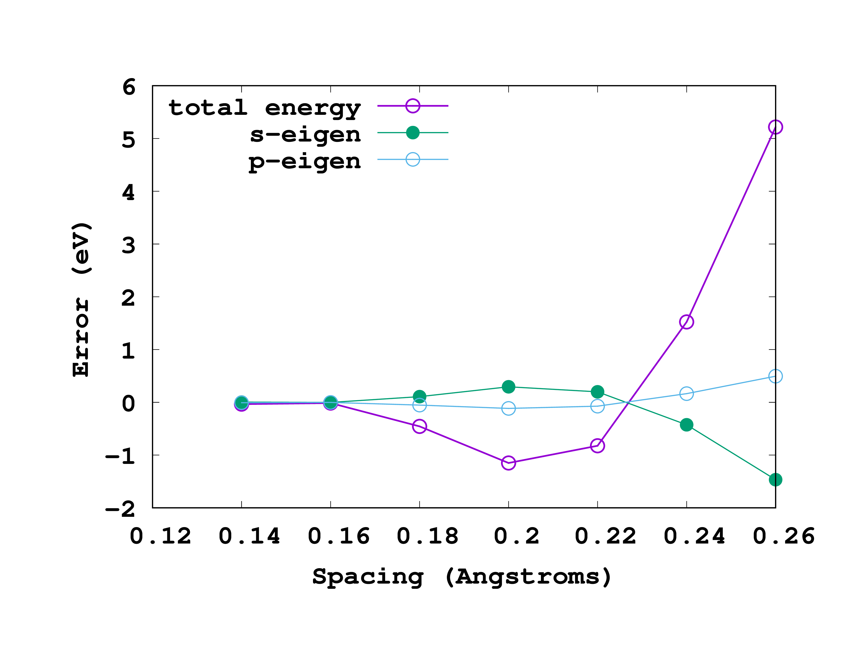
The results, for this particular example, are shown in the figure. In this figure we are actually plotting the error with respect to the most accurate results (smallest spacing). That means that we are plotting the ‘‘‘difference’’’ between the values for a given spacing and the values for a spacing of 0.14 Å. So, in reading it, note that the most accurate results are at the left (smallest spacing). A rather good spacing for this nitrogen pseudopotential seems to be 0.18 Å. However, as we are usually not interested in total energies, but in energy differences, probably a larger one may also be used without compromising the results.
Methane molecule
We will now move on to a slightly more complex system, the methane molecule CH4, and add a convergence study with respect to the box size.
Input
As usual, the first thing to do is create an input file for this system. From our basic chemistry class we know that methane has a tetrahedral structure. The only other thing required to define the geometry is the bond length between the carbon and the hydrogen atoms. If we put the carbon atom at the origin, the hydrogen atoms have the coordinates given in the following input file:
CalculationMode = gs
UnitsOutput = eV_Angstrom

FromScratch = yes

Radius = 3.5*angstrom
Spacing = 0.22*angstrom

CH = 1.2*angstrom
%Coordinates
 "C" |           0 |          0 |           0
 "H" |  CH/sqrt(3) | CH/sqrt(3) |  CH/sqrt(3)
 "H" | -CH/sqrt(3) |-CH/sqrt(3) |  CH/sqrt(3)
 "H" |  CH/sqrt(3) |-CH/sqrt(3) | -CH/sqrt(3)
 "H" | -CH/sqrt(3) | CH/sqrt(3) | -CH/sqrt(3)
%

EigenSolver = chebyshev_filter
ExtraStates = 4
# Restart data from this run is not read by any later step of this test.
RestartWrite = no
Here we define a variable CH that represents the bond length between the carbon and the hydrogen atoms, which simplifies the writing of the coordinates. We start with a bond length of 1.2 Å but that’s not so important at the moment, since we can optimize it later (for more information see the Geometry optimization tutorial). (You should not use 5 Å or so, but something slightly bigger than 1 Å is fine.)
Some notes concerning the input file:
- We do not tell Octopus explicitly which BoxShape to use. The default is a union of spheres centered around each atom. This turns out to be the most economical choice in almost all cases.
- We also do not specify the %Species block. In this way, Octopus will use default pseudopotentials for both Carbon and Hydrogen. This should be OK in many cases, but, as a rule of thumb, you should do careful testing before using any pseudopotential for serious calculations.
If you use the given input file you should find the following values in the resulting static/info file.
Eigenvalues [eV]
 #st  Spin   Eigenvalue      Occupation
   1   --   -15.990990       2.000000
   2   --    -9.065638       2.000000
   3   --    -9.065638       2.000000
   4   --    -9.065638       2.000000
   5   --     0.267941       0.000000
   6   --     1.928187       0.000000
   7   --     1.928187       0.000000
   8   --     1.928187       0.000000

Energy [eV]:
      Total       =      -219.03767589
      Free        =      -219.03767589
      -----------
      Ion-ion     =       236.08498119
      Eigenvalues =       -86.37580557
      Hartree     =       393.45810130
      Int[n*v_xc] =      -105.38066063
      Exchange    =       -69.66883931
      Correlation =       -11.00057152
      vanderWaals =         0.00000000
      Delta XC    =         0.00000000
      Entropy     =         0.00000000
      -TS         =        -0.00000000
      Photon ex.  =         0.00000000
      Kinetic     =       163.97241304
      External    =      -931.88367517
      Non-local   =       -49.75780023
      Int[n*v_E]  =         0.00000000
Now the question is whether these values are converged or not. This will depend on two things: the Spacing, as seen above, and the Radius. Just like for the Nitrogen atom, the only way to answer this question is to try other values for these variables.
Convergence with the spacing
As before, we will keep all entries in the input file fixed except for the spacing that we will make smaller by 0.02 Å all the way down to 0.1 Å. So you have to run Octopus several times. You can use a similar script as the one from the Nitrogen atom example:
#!/bin/bash
echo "#Sp    Energy" > spacing.dat
list="0.22 0.20 0.18 0.16 0.14 0.12 0.10"
export OCT_PARSE_ENV=1
for Spacing in $list
do
    export OCT_Spacing=$(echo $Spacing*1.8897261328856432 | bc)
    octopus >& out-$Spacing
    energy=`grep Total static/info  | head -1 | cut -d "=" -f 2`
    echo $Spacing $energy >> spacing.dat
    rm -rf restart
done
 unset OCT_Spacing
For this example we changed the list of spacings to try and, to keep things simple, we are only writing the total energy to the spacing.dat file.
Now run the script to get the following results:
#Sp    Energy
0.22 -219.03767589
0.20 -218.58409056
0.18 -218.27963068
0.16 -218.20008101
0.14 -218.17904584
0.12 -218.15967953
0.10 -218.13929288
If you give these numbers to ‘‘gnuplot’’ (or other software to plot) you will get a curve like the one shown below:
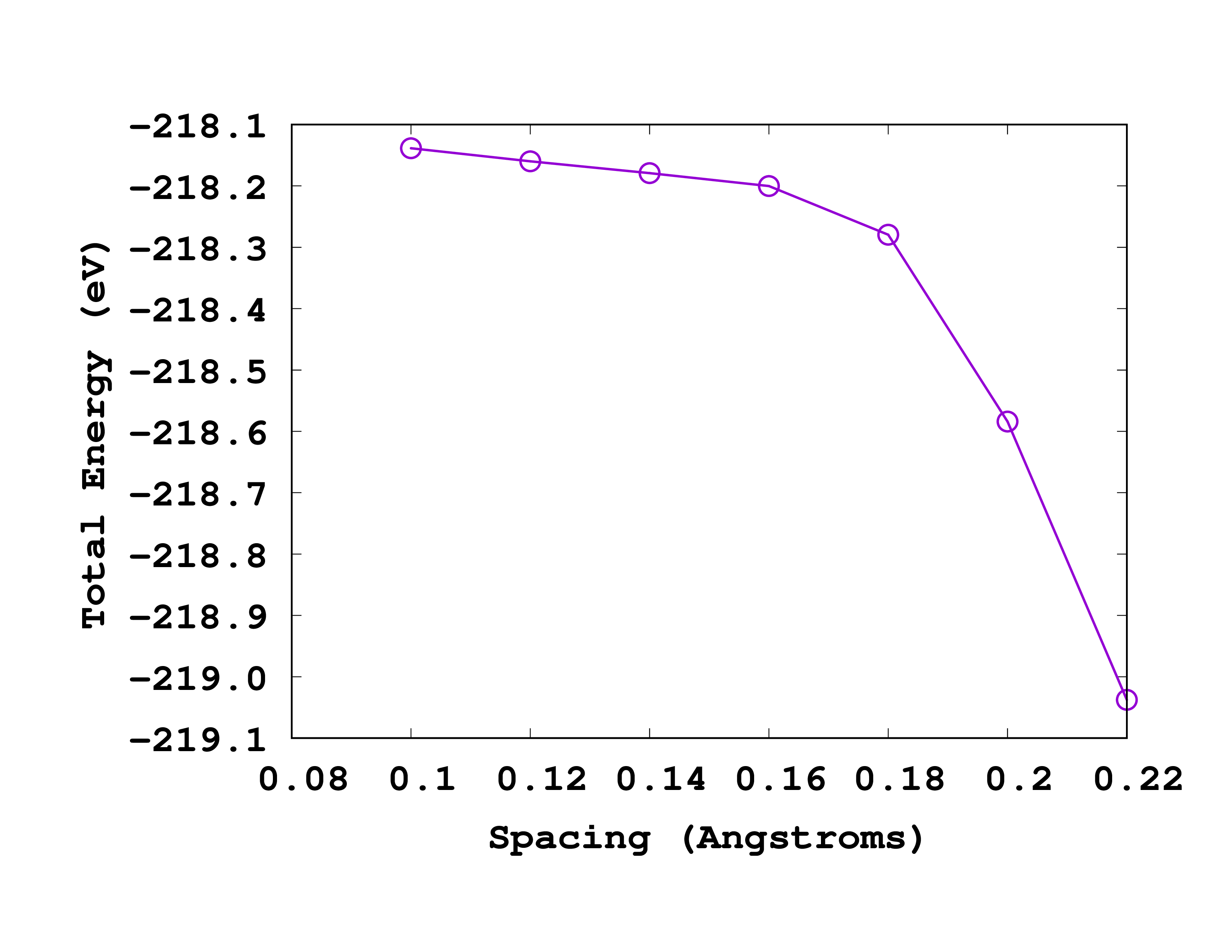
As you can see from this picture, the total energy is converged to within 0.1 eV for a spacing of 0.18 Å. So we will use this spacing for the next calculations.
Convergence with the radius
Now we will see how the total energy changes with the Radius of the box. We will change the radius in steps of 0.5 Å. You can change the input file by hand and run Octopus each time, or again use a small script:
#!/bin/bash
echo "#Rad   Energy" > radius.dat
list="2.5 3.0 3.5 4.0 4.5 5.0"
export OCT_PARSE_ENV=1
for Radius in $list
do
    export OCT_Radius=$(echo $Radius*1.8897261328856432 | bc)
    octopus >& out-$Radius
    energy=`grep Total static/info  | head -1 | cut -d "=" -f 2`
    echo $Radius $energy >> radius.dat
    rm -rf restart
done
unset OCT_Radius
Before running the script, make sure that the spacing is set to 0.18 Å in the input file. You should then get a file radius.dat that looks like this:
#Rad   Energy
2.5 -218.07115147
3.0 -218.24555504
3.5 -218.27963068
4.0 -218.28620504
4.5 -218.28758540
5.0 -218.28784961
Below you can see how this looks like when plotted. Note that in this case, the most accurate results are on the right (larger radius).
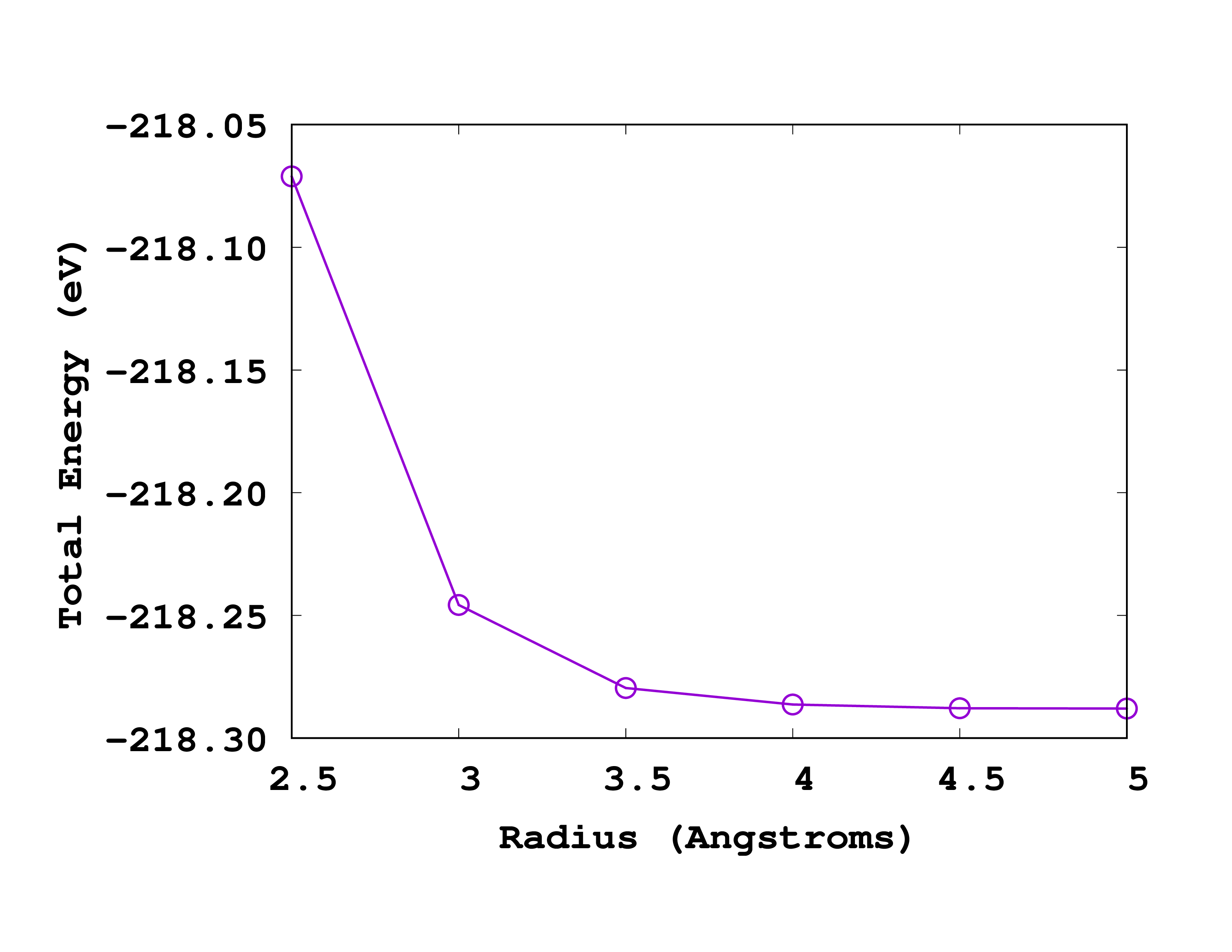
If we again ask for a convergence up to 0.1 eV we should use a radius of 3.5 Å. How does this compare to the size of the molecule? Can you explain why the energy increases (becomes less negative) when one decreases the size of the box?