1D Harmonic Oscillator
As a first example we use the standard textbook harmonic oscillator in one dimension and fill it with two non-interacting electrons.
Input
The first thing to do is to tell Octopus what we want it to do. Write the following lines and save the file as inp .
FromScratch = yes
CalculationMode = gs

Dimensions = 1
TheoryLevel = independent_particles

Radius = 10
Spacing = 0.1

%Species
  "HO" | species_user_defined | potential_formula | "0.5*x^2" | valence | 2
%

%Coordinates
  "HO" | 0
%

Eigensolver = chebyshev_filter
ExtraStates = 2
Most of these input variables should already be familiar. Here is a more detailed explanation for some of the values:
-
Dimensions = 1: This means that the code should run for 1-dimensional systems. Other options are 2, or 3 (the default). You can actually run in 4D too if you have compiled with the configure flag –max-dim=4. -
TheoryLevel = independent_particles: We tell Octopus to treat the electrons as non-interacting. -
Radius = 10.0: The radius of the 1D “sphere,” ‘‘i.e.’’ a line; therefore domain extends from -10 to +10 bohr. -
%Species: The species name is “HO”, then the potential formula is given, and finally the number of valence electrons. See Input file for a description of what kind of expressions can be given for the potential formula. -
%Coordinates: add the external potential defined for species “HO” in the position (0,0,0). The coordinates used in the potential formula are relative to this point.
Output
Now one can execute this file by running Octopus. Here are a few things worthy of a closer look in the standard output.
First one finds the listing of the species:
****************************** Species *******************************
Species "HO" is a user-defined potential.
   Potential = 0.5*x^2
Number of orbitals:      5
**********************************************************************
The potential is $V(x) = 0.5 x^2$, and 5 Hermite-polynomial orbitals are available for LCAO (the number is based on the valence). The theory level is as we requested:
**************************** Theory Level ****************************
Input: [TheoryLevel = independent_particles]
**********************************************************************
The electrons are treated as “non-interacting”, which means that the Hartree and exchange-correlation terms are not included. This is usually appropriate for model systems, in particular because the standard XC approximations we use for actual electrons are not correct for “effective electrons” with a different mass.
Input: [MixField = none] (what to mix during SCF cycles)
Since we are using independent particles (and only one electron) there is no need to use a mixing scheme to accelerate the SCF convergence. Apart from these differences, the calculation follows the same pattern as in the Getting Started tutorial and converges after a few iterations:
*********************** SCF CYCLE ITER #    8 ************************
 etot  =  1.00000000E+00 abs_ev   =  2.41E-13 rel_ev   =  2.41E-13
 ediff =        2.41E-13 abs_dens =  2.94E-07 rel_dens =  1.47E-07
Matrix vector products:     25
Converged eigenvectors:      0

#  State  Eigenvalue [H]  Occupation    Error
      1        0.500000    2.000000   ( 2.2E-07)
      2        1.500000    0.000000   ( 7.6E-05)
      3        2.506453    0.000000   ( 1.7E-01)

Density of states:

%---------------------------------%----------------------------------%
%---------------------------------%----------------------------------%
%---------------------------------%----------------------------------%
%---------------------------------%----------------------------------%
%---------------------------------%----------------------------------%
%---------------------------------%----------------------------------%
%---------------------------------%----------------------------------%
%---------------------------------%----------------------------------%
%---------------------------------%----------------------------------%
%---------------------------------%----------------------------------%
^


Elapsed time for SCF step     8:          0.00
**********************************************************************
Note that, as the electrons are non-interacting, there is actually no self-consistency needed. Nevertheless, Octopus takes several SCF iterations to converge. This is because it takes more than one SCF iteration for the iterative eigensolver to converge the wave-functions and eigenvalues.
Exercises
The first thing to do is to look at the static/info file. Look at the eigenvalue and total energy. Compare to your expectation from the analytic solution to this problem!
We can also play a little bit with the input file and add some other features. For example, what about the other eigenstates of this system? To obtain them we can calculate some unoccupied states. This can be done by changing the CalculationMode to
CalculationMode = unocc
in the input file. In this mode Octopus will not only give you the occupied states (which contribute to the density) but also the unoccupied ones. Set the number of states with an extra lines
 ExtraStatesToConverge = 10
 ExtraStates = 12
that will calculate 12 empty states and treat the last two as buffer. Indeed, as we are using the eigensolver chebyshev_filter, we need to add a few more extra states, which do not have to be converged. For more detail, see the manual page on eigensolvers.
A thing to note here is that Octopus will need the density for this calculation. (Actually for non-interacting electrons the density is not needed for anything, but since Octopus is designed for interacting electrons it will try to read the density anyways.) So if you have already performed a static calculation (CalculationMode = gs) it will just use this result.
Compared to the ground-state calculation we also have to change the convergence criterion. The unoccupied states do not contribute to the density so they might not (and actually will not) converge properly if we use the density for the convergence check. Therefore, Octopus now checks whether all calculated states converge separately by just looking at the biggest error in the wave-functions. From the calculation you get another file in the static directory called eigenvalues . The info file will only contain the information about the ground-state; all eigenvalues and occupation numbers will be in the eigenvalues file.
If we also want to plot, say, the wave-function, at the end of the calculation, we have to tell Octopus to give us this wave-function and how it should do this. We just include
 %Output
    wfs
 %
 OutputFormat = axis_x
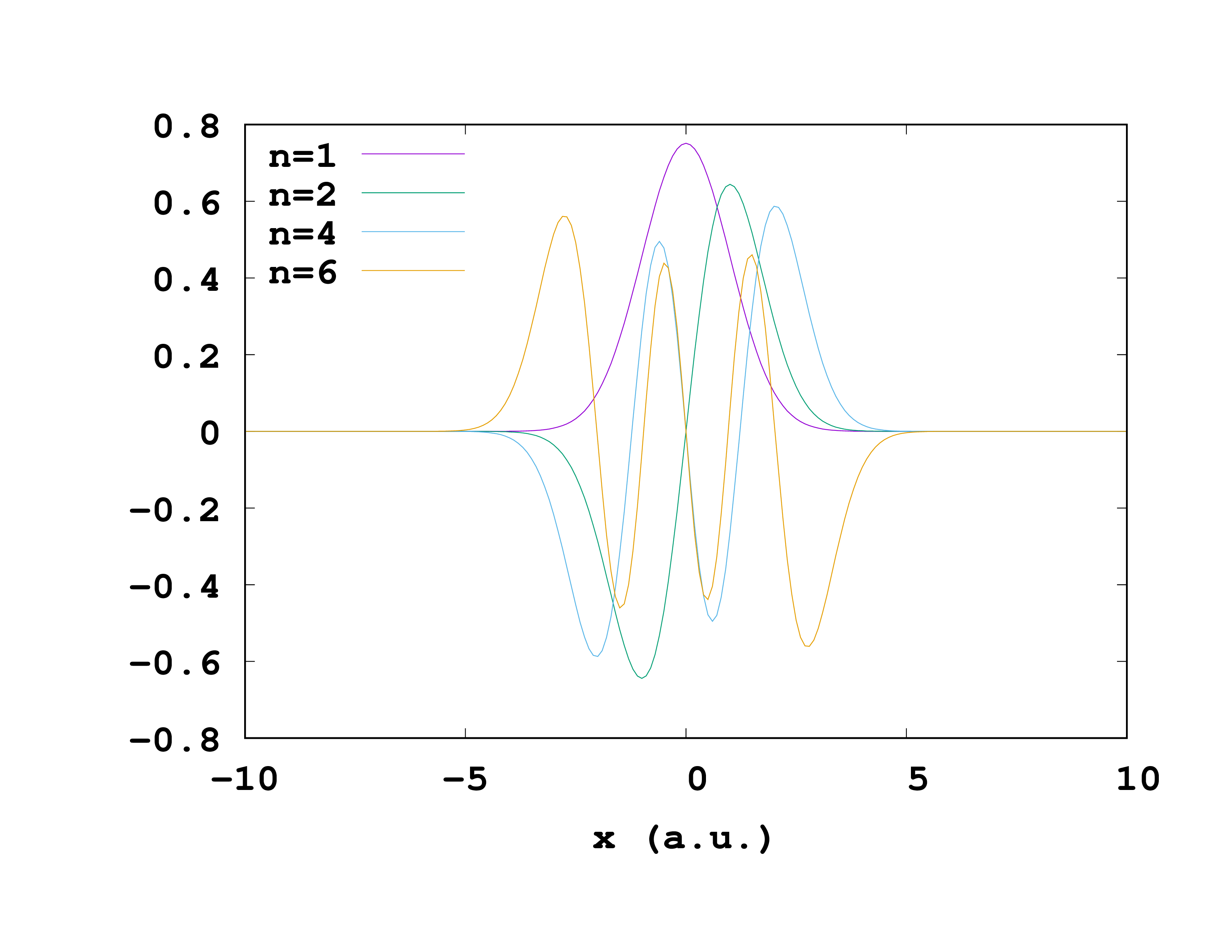
The first line tells Octopus to give out the wave-functions and the second line says it should do so along the x-axis. We can also select the wave-functions we would like as output, for example the first and second, the fourth and the sixth. (If you don’t specify anything Octopus will give them all.)
OutputWfsNumber = "1-2,4,6"
Octopus will store the wave-functions in the same folder static where the info file is, under a meaningful name. They are stored as pairs of the ‘‘x’’-coordinate and the value of the wave-function at that position ‘‘x’’. One can easily plot them with gnuplot or a similar program.
It is also possible to extract a couple of other things from Octopus like the density or the Kohn-Sham potential.