Visualization
In this tutorial we will explain how to visualize outputs from Octopus. Several different file formats are available in Octopus that are suitable for a variety of visualization software. We will not cover all of them here. See Visualization for more information.
Benzene molecule
As an example, we will use the benzene molecule. At this point, the input should be quite familiar to you:
CalculationMode = gs
UnitsOutput = eV_Angstrom

Radius = 5*angstrom
Spacing = 0.15*angstrom

%Output
  wfs
  density
  elf
  potential
%

OutputFormat = cube + xcrysden + dx + axis_x + plane_z

XYZCoordinates = "benzene.xyz"

EigenSolver = chebyshev_filter
ExtraStates = 4
Coordinates are in this case given in the benzene.xyz file. This file should look like:
12
   Geometry of benzene (in Angstrom)
   C  0.000  1.396  0.000
   C  1.209  0.698  0.000
   C  1.209 -0.698  0.000
   C  0.000 -1.396  0.000
   C -1.209 -0.698  0.000
   C -1.209  0.698  0.000
   H  0.000  2.479  0.000
   H  2.147  1.240  0.000
   H  2.147 -1.240  0.000
   H  0.000 -2.479  0.000
   H -2.147 -1.240  0.000
   H -2.147  1.240  0.000
Here we have used two new input variables:
- Output: this tells Octopus what quantities to output.
- OutputFormat: specifies the format of the output files.
In this case we ask Octopus to output the wavefunctions (wfs), the density, the electron localization function (elf) and the Kohn-Sham potential. We ask Octopus to generate this output in several formats, that are required for the different visualization tools that we mention below. If you want to save some disk space you can just keep the option that corresponds to the program you will use. Take a look at the documentation on variables Output and OutputFormat for the full list of possible quantities to output and formats to visualize them in.
If you now run Octopus with this input file, you should get the following files in the static directory:
 %ls static
 convergence      forces      vh.z=0       wf-st0001.cube     wf-st0003.dx       wf-st0005.xsf      wf-st0007.y=0,z=0  wf-st0009.z=0      wf-st0012.cube     wf-st0014.dx
 density.cube     info        vks.cube     wf-st0001.dx       wf-st0003.xsf      wf-st0005.y=0,z=0  wf-st0007.z=0      wf-st0010.cube     wf-st0012.dx       wf-st0014.xsf
 density.dx       v0.cube     vks.dx       wf-st0001.xsf      wf-st0003.y=0,z=0  wf-st0005.z=0      wf-st0008.cube     wf-st0010.dx       wf-st0012.xsf      wf-st0014.y=0,z=0
 density.xsf      v0.dx       vks.xsf      wf-st0001.y=0,z=0  wf-st0003.z=0      wf-st0006.cube     wf-st0008.dx       wf-st0010.xsf      wf-st0012.y=0,z=0  wf-st0014.z=0
 density.y=0,z=0  v0.xsf      vks.y=0,z=0  wf-st0001.z=0      wf-st0004.cube     wf-st0006.dx       wf-st0008.xsf      wf-st0010.y=0,z=0  wf-st0012.z=0      wf-st0015.cube
 density.z=0      v0.y=0,z=0  vks.z=0      wf-st0002.cube     wf-st0004.dx       wf-st0006.xsf      wf-st0008.y=0,z=0  wf-st0010.z=0      wf-st0013.cube     wf-st0015.dx
 elf_rs.cube      v0.z=0      vxc.cube     wf-st0002.dx       wf-st0004.xsf      wf-st0006.y=0,z=0  wf-st0008.z=0      wf-st0011.cube     wf-st0013.dx       wf-st0015.xsf
 elf_rs.dx        vh.cube     vxc.dx       wf-st0002.xsf      wf-st0004.y=0,z=0  wf-st0006.z=0      wf-st0009.cube     wf-st0011.dx       wf-st0013.xsf      wf-st0015.y=0,z=0
 elf_rs.xsf       vh.dx       vxc.xsf      wf-st0002.y=0,z=0  wf-st0004.z=0      wf-st0007.cube     wf-st0009.dx       wf-st0011.xsf      wf-st0013.y=0,z=0  wf-st0015.z=0
 elf_rs.y=0,z=0   vh.xsf      vxc.y=0,z=0  wf-st0002.z=0      wf-st0005.cube     wf-st0007.dx       wf-st0009.xsf      wf-st0011.y=0,z=0  wf-st0013.z=0
 elf_rs.z=0       vh.y=0,z=0  vxc.z=0      wf-st0003.cube     wf-st0005.dx       wf-st0007.xsf      wf-st0009.y=0,z=0  wf-st0011.z=0      wf-st0014.cube
Visualization
Post-processing of the data generated by Octopus can be done in many different ways.
Here we will introduce some of the most common tools including postopus which is a python tool developed primarily for the POST-processing of octOPUS data.
Postopus
Postopus can be installed using pip install postopus[recommended] on a command line.
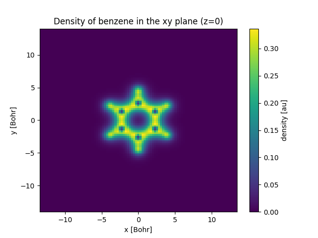
A sample program to plot a slice density of benzene in the xy plane (z=0) is shown below:
import matplotlib.pyplot as plt
import postopus

run = postopus.Run("/path/to/octopus/run")
density = run.default.scf.density(source="cube")
density.sel(z=0, method="nearest").plot(x="x")
plt.title("Density of benzene in the xy plane (z=0)")
plt.savefig("benzene_density.pdf")
More information about postopus can be found in the postopus documentation. This example is covered in more detail here and a quick start for postopus is available here.
Gnuplot
Visualization of the fields in 3-dimensions is complicated. In many cases it is more useful to plot part of the data, for example the values of a scalar field along a line of plane that can be displayed as a 1D or 2D plot.
The gnuplot program is very useful for making these types of plots (and many more) and can directly read Octopus output. First type gnuplot to enter the program’s command line. Now to plot a the density along a line (the X axis in this case) type
plot "static/density.y=0,z=0" w l
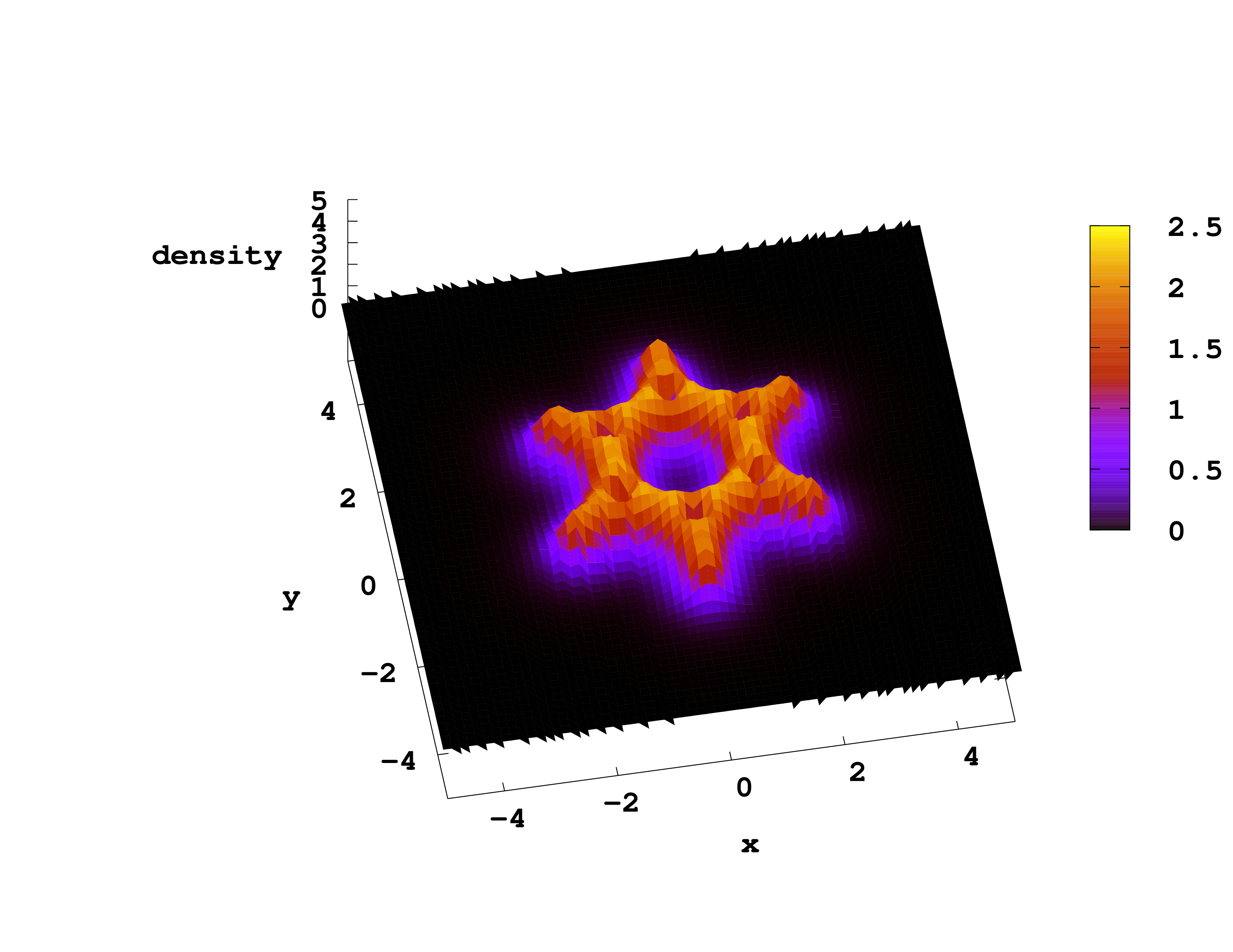
To plot a 2D field, for example the density in the plane z=0, you can use the command
splot "static/density.z=0" w l
If you want to get a color scale for the values of the field use “w pm3d” instead of “w l”.
VisIt
The program VisIt is an open-source data visualizer developed by Lawrence Livermore National Laborartory. It supports multiple platforms including Linux, OS X and Windows, most likely you can download a precompiled version for your platform here.
For this tutorial you need to have Visit installed and running. VisIt can read several formats, the most convenient for Octopus data is the cube format: OutputFormat = cube. This is a common format that can be read by several visualization and analysis programs, it has the advantage that includes both the requested scalar field and the geometry in the same file. Visit can also read other formats that Octopus can generate like xyz, XSF (partial support), and VTK.
The following video contains the instruction on how to open a cube file in VisIt. Note that the video has subtitles in case you don’t have audio in your current location, you can enable them by clicking the “CC” button.
XCrySDen
Atomic coordinates (finite or periodic), forces, and functions on a grid can be plotted with the free program XCrysDen. Its XSF format also can be read by V_Sim and VESTA. Beware, these all probably assume that your output is in Angstrom units (according to the specification), so use UnitsOutput = eV_Angstrom, or your data will be misinterpreted by the visualization software.
UCSF Chimera
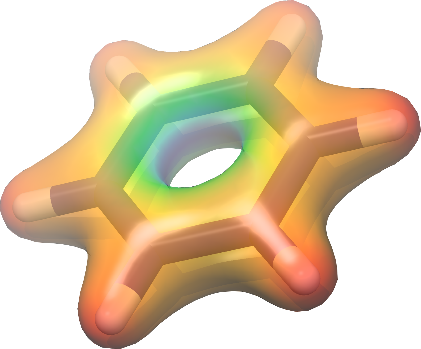
Those .dx files can be also be opened by UCSF Chimera .
Once having UCSF Chimera installed and opened, open the benzene.xyz file from ‘‘‘File > Open’’’.
To open the .dx file, go to ‘‘‘Tools > Volume Data > Volume Viewer’’’. A new window opens. There go to ‘‘‘File > Open’’’ and select static/density.dx .
To “color” the density go to ‘‘‘Tools > Surface Color’’’. A new dialog opens and there choose ‘‘‘Browse’’’ to open the vh.dx file. Then click ‘‘‘Color’’’ and you should have an image similar to the below one.