Time-dependent propagation
OK, it is about time to do TDDFT. Let us perform a calculation of the time evolution of the density of the methane molecule.
Ground-state
The reason to do first a ground-state DFT calculation is that this will be the initial state for the real-time calculation.
Run the input file below to obtain a proper ground-state (stored in the restart directory) as from the
total energy convergence tutorial. (Now we are using a more accurate bond length than before.)
CalculationMode = gs
UnitsOutput = eV_Angstrom

Radius = 3.5*angstrom
Spacing = 0.18*angstrom

CH = 1.097*angstrom
%Coordinates
  "C" |           0 |          0 |           0
  "H" |  CH/sqrt(3) | CH/sqrt(3) |  CH/sqrt(3)
  "H" | -CH/sqrt(3) |-CH/sqrt(3) |  CH/sqrt(3)
  "H" |  CH/sqrt(3) |-CH/sqrt(3) | -CH/sqrt(3)
  "H" | -CH/sqrt(3) | CH/sqrt(3) | -CH/sqrt(3)
%

Eigensolver = chebyshev_filter
ExtraStates = 4
Time-dependent
Input
Now that we have a starting point for our time-dependent calculation, we modify the input file so that it looks like this:
CalculationMode = td
UnitsOutput = eV_Angstrom

Radius = 3.5*angstrom
Spacing = 0.18*angstrom

CH = 1.097*angstrom
%Coordinates
  "C" |           0 |          0 |           0
  "H" |  CH/sqrt(3) | CH/sqrt(3) |  CH/sqrt(3)
  "H" | -CH/sqrt(3) |-CH/sqrt(3) |  CH/sqrt(3)
  "H" |  CH/sqrt(3) |-CH/sqrt(3) | -CH/sqrt(3)
  "H" | -CH/sqrt(3) | CH/sqrt(3) | -CH/sqrt(3)
%

Tf  = 0.1/eV
dt = 0.002/eV

TDPropagator = aetrs
TDMaxSteps = Tf/dt
TDTimeStep = dt


# Restart data from this run is not read by any later step of this test.
RestartWrite = no
Here we have switched on a new run mode, CalculationMode = td instead of gs, to do a time-dependent run. We have also added three new input variables:
-
TDPropagator: which algorithm will be used to approximate the evolution operator. Octopus has a large number of possible propagators that you can use (see Ref.1 for an overview).
-
TDMaxSteps: the number of time-propagation steps that will be performed.
-
TDTimeStep: the length of each time step.
Note that, for convenience, we have previously defined a couple of variables, Tf and dt. We have made use of one of the possible propagators, aetrs. The manual explains about the possible options; in practice this choice is usually good except for very long propagation where the etrs propagator can be more stable.
Output
Now run Octopus. This should take a few seconds, depending on the speed of your machine. The most relevant chunks of the standard output are
Input: [IonsConstantVelocity = no]
Input: [Thermostat = none]
Input: [MoveIons = no]
Input: [TDTimeStep = 0.2000E-02 hbar/eV]
Input: [TDPropagationTime = 0.1000 hbar/eV]
Input: [TDMaxSteps = 50]
Input: [TDDynamics = ehrenfest]
Input: [TDScissor = 0.000]
Input: [TDPropagator = aetrs]
Input: [TDExponentialMethod = taylor]
********************* Time-Dependent Simulation **********************
  Iter           Time        Energy   SC Steps    Elapsed Time
**********************************************************************

      1       0.002000   -218.870493         1         0.072
      2       0.004000   -218.870493         1         0.069
      3       0.006000   -218.870493         1         0.069
...

     48       0.096000   -218.870493         1         0.069
     49       0.098000   -218.870493         1         0.071
     50       0.100000   -218.870493         1         0.077
It is worthwhile to comment on a few things:
- We have just performed the time-evolution of the system, departing from the ground-state, under the influence of no external perturbation. As a consequence, the electronic system does not evolve. The total energy does not change (this you may already see in the output file, the third column of numbers), nor should any other observable change. However, this kind of run is useful to check that the parameters that define the time evolution are correct.
- As the evolution is performed, the code probes some observables and prints them out. These are placed in some files under the directory td.general
, which should show up in the working directory. In this case, only two files show up, the td.general/energy
, and the td.general/multipoles
files. The td.general/multipoles
file contains a large number of columns of data. Each line corresponds to one of the time steps of the evolution (except for the first three lines, that start with a
-symbol, which give the meaning of the numbers contained in each column, and their units). A brief overview of the information contained in this file follows:- The first column is just the iteration number.
- The second column is the time.
- The third column is the dipole moment of the electronic system, along the $x$-direction: $\langle \Phi (t) \vert \hat{x} \vert \Phi(t)\rangle = \int\!\!{\rm d}^3r\; x\,n(r)$. Next are the $y$- and $z$-components of the dipole moment.
- The file td.general/energy contains the different components of the total energy.
- It is possible to restart a time-dependent run. Try that now. Just increase the value of TDMaxSteps and rerun Octopus. If, however, you want to start the evolution from scratch, you should set the variable FromScratch to
yes.
The time step
A key parameter is, of course, the time step, TDTimeStep. Before making long calculations, it is worthwhile spending some time choosing the largest time-step possible, to reduce the number of steps needed. This time-step depends crucially on the system under consideration, the spacing, on the applied perturbation, and on the algorithm chosen to approximate the evolution operator.
In this example, try to change the time-step and to rerun the time-evolution. Make sure you are using TDMaxSteps of at least 100, as with shorter runs an instability might not appear yet. You will see that for time-steps larger than 0.0024 the propagation gets unstable and the total energy of the system is no longer conserved. Very often it diverges rapidly or even becomes NaN.
Also, there is another input variable that we did not set explicitly, relying on its default value, TDExponentialMethod. Since most propagators rely on algorithms to calculate the action of the exponential of the Hamiltonian, one can specify which algorithm can be used for this purpose.
You may want to learn about the possible options that may be taken by TDExponentialMethod, and TDPropagator – take a look at the manual. You can now try some exercises:
-
Fixing the propagator algorithm (for example, to the default value), investigate how the several exponentiation methods work (Taylor, Chebyshev, and Lanczos). This means finding out what maximum time-step one can use without compromising the proper evolution.
-
And fixing now the TDExponentialMethod, one can now play around with the various propagators.
Laser fields
Now we will add a time-dependent external perturbation (a laser field) to the molecular Hamiltonian. For brevity, we will omit the beginning of the file, as this is left unchanged. The relevant part of the input file, with the modifications and additions is:
Tf  = 1/eV
dt = 0.002/eV

TDPropagator = aetrs
TDMaxSteps = Tf/dt
TDTimeStep = dt

FromScratch = yes

amplitude = 1*eV/angstrom
omega = 18.0*eV
tau0 = 0.5/eV
t0 = tau0

%TDExternalFields
  electric_field | 1 | 0 | 0 | omega | "envelope_cos"
%

%TDFunctions
  "envelope_cos" | tdf_cosinoidal | amplitude | tau0 | t0
%

%TDOutput
 laser
 multipoles
%
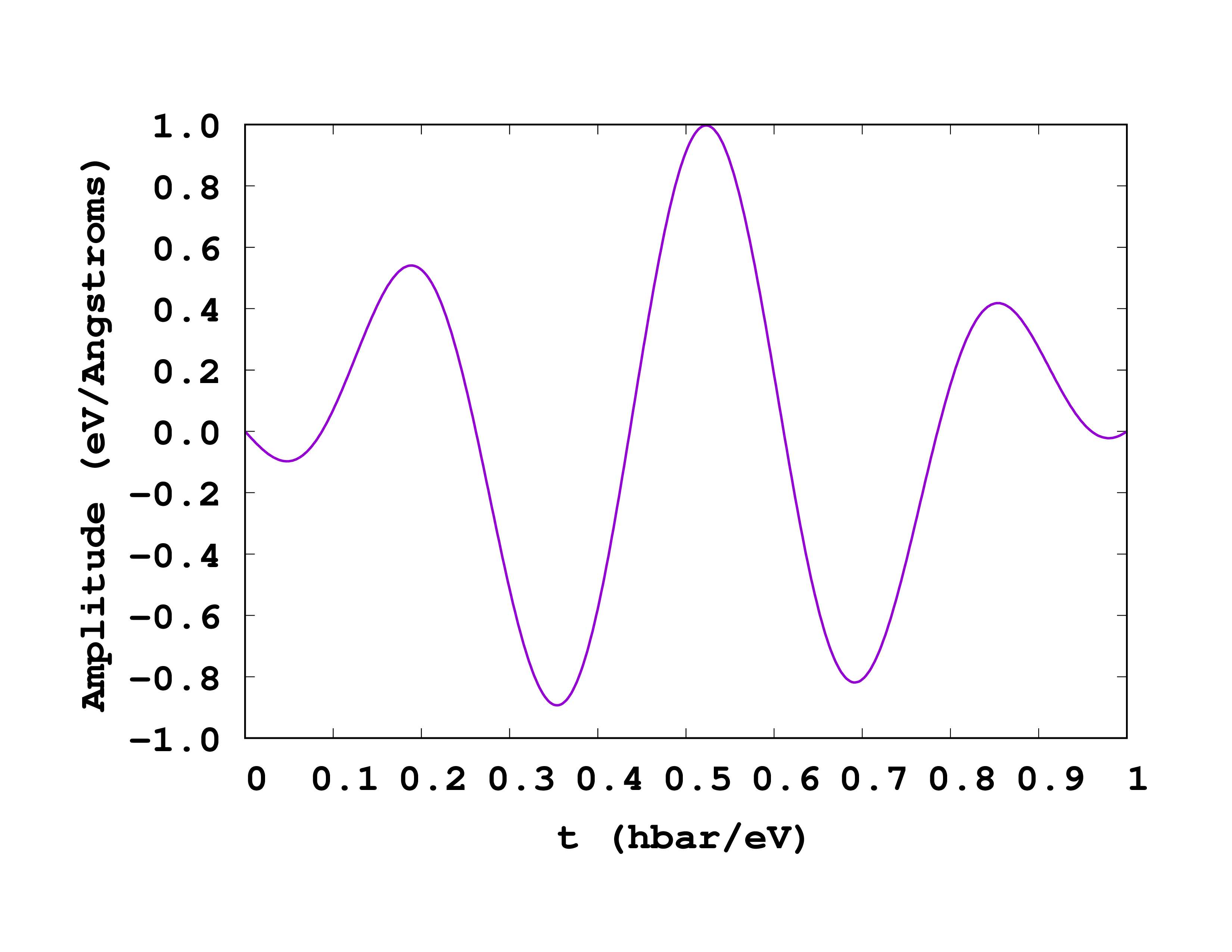
The most important variables here are the TDExternalFields block and the associated TDFunctions block. You should carefully read the manual page dedicated to these variables: the particular laser pulse that we have employed is the one whose envelope function is a cosine.
Now you are ready to set up a run with a laser field. Be careful to set a total time of propagation able to accommodate the laser shot, or even more if you want to see what happens afterwards. You may also want to consult the meaning of the variable TDOutput.
A couple of important comments:
- You may supply several laser pulses: simply add more lines to the TDExternalFields block and, if needed, to the TDFunctions block.
- We have added the
laseroption to TDOutput variable, so that the laser field is printed in the file td.general/laser . This is done immediately at the beginning of the run, so you can check that the laser is correct without waiting. - You can have an idea of the response to the field by looking at the dipole moment in the td.general/multipoles . What physical observable can be calculated from the response?
- When an external field is present, one may expect that unbound states may be excited, leading to ionization. In the calculations, this is reflected by density reaching the borders of the box. In these cases, the proper way to proceed is to setup absorbing boundaries (variables AbsorbingBoundaries, ABWidth and ABCapHeight).
-
A. Castro, M.A.L. Marques, and A. Rubio, Propagators for the time-dependent Kohn–Sham equations, J. Chem. Phys. 121 3425-3433 (2004); ↩︎