Navigation :
Manual
Input Variables
Tutorials
-
Octopus Basics
-
Optical Response
-
Periodic Systems
-
Model Systems
-
Running Octopus on HPC systems
-
Maxwell Systems
-- Maxwell input file
-- Plane waves in vacuum
-- External currents and PML
-- Non-dispersive linear media
-- Dispersive linear media
-
Multisystem
- CECAM workshop April 2024
-
Advanced tutorials
-
Courses
Developers
Releases
Dispersive linear media
In addition to the possibility to include objects described as static linear
media, Octopus allows for simulations with dispersive media. For example, let’s
consider the following input file, for propagation of a pulse through a sphere
described by a Drude polarizability:
CalculationMode = td
ExperimentalFeatures = yes
Restartwalltimeperiod = 1.1
%Systems
 'Maxwell' | maxwell
 'NP' | dispersive_medium
%

 MediumPoleEnergy = 9.03*ev
 MediumPoleDamping = 0.053*ev
 MediumDispersionType = drude_medium
 %MediumCurrentCoordinates
   -160.0*nm | 0.0 | 0.0
   -80.0*nm | 0.0 | 0.0
%
# ----- Maxwell box variables ---------------------------------------------------------------------

 l_zero = 550*nm     #central wavelength
 lsize_mx = 1.25*l_zero
 lsize_myz = 0.5*l_zero
 S_c = 0.2 ##Courant condition coefficient

 dx_mx    = 20*nm
 BoxShape   = parallelepiped
 NP.BoxShape = box_cgal
 NP.BoxCgalFile = "gold-np-r80nm.off"

%Lsize
 lsize_mx+0.25*l_zero | lsize_myz+0.25*l_zero | lsize_myz+0.25*l_zero
%

%Spacing
 dx_mx | dx_mx | dx_mx
%

%MaxwellBoundaryConditions
 plane_waves | zero | zero
%

%MaxwellAbsorbingBoundaries
 cpml | cpml | cpml
%

MaxwellABWidth              = 0.25*l_zero
MaxwellABPMLPower           = 3.0
MaxwellABPMLReflectionError = 1e-16

OutputFormat = axis_x + plane_y

%MaxwellOutput
 electric_field
 total_current_mxll
%

MaxwellOutputInterval = 20
MaxwellTDOutput       = maxwell_energy + maxwell_total_e_field

%MaxwellFieldsCoordinate
  -120.0*nm | 0.0 | 0.0
  -80.0*nm | 0.0 | 0.0
  -20.0*nm | 0.0 | 0.0
%

Maxwell.TDSystemPropagator = prop_expmid
NP.TDSystemPropagator      = prop_rk4

timestep                = S_c*dx_mx/c
TDTimeStep              = timestep
TDPropagationTime       = 240*timestep

lambda = l_zero
omega  = 2 * pi * c / lambda
kx     = omega / c
Ez    = 1.0
sigma = 40.0*c
p_s     = -lsize_mx*1.2

%UserDefinedInitialMaxwellStates
 use_incident_waves
%

%MaxwellIncidentWaves
 plane_wave_mx_function | electric_field | 0 | 0 | Ez | "plane_waves_function"
%

%MaxwellFunctions
 "plane_waves_function" | mxf_gaussian_wave | kx | 0 | 0 | p_s | 0 | 0 | sigma
%
Here, we need to define the variables MediumPoleEnergy and
MediumPoleDamping , which represent the plasma frequency $\omega_p$ and
inverse lifetime $\gamma$ of a Drude pole. For this example, the parameters are those
for the Drude peak of gold, as taken from the literature MediumCurrentCoordinates to obtain the
polarization current at certain points. The rest of the input variables of
the medium are the same that have been used for the static linear medium. In
this case, we are using an off file that contains the shape of a sphere of 80
nm radius, which is displaced from the origin by one radius to the negative x
direction.
off file
OFF

450 896 0
-3023.52 0 0
-2990.48 -314.31299 0
-2990.48 0 -314.31299
-2990.48 0 314.31299
-2990.48 314.31299 0
-2958.1699 -307.444 -314.31299
-2958.1699 -307.444 314.31299
-2958.1699 307.444 -314.31299
-2958.1699 307.444 314.31299
-2892.8201 -614.888 0
-2892.8201 0 -614.888
-2892.8201 0 614.888
-2892.8201 614.888 0
-2862.6399 -601.45099 -314.31299
-2862.6399 -601.45099 314.31299
-2862.6399 -287.13901 -614.888
-2862.6399 -287.13901 614.888
-2862.6399 287.13901 -614.888
-2862.6399 287.13901 614.888
-2862.6399 601.45099 -314.31299
-2862.6399 601.45099 314.31299
-2773.4199 -561.72803 -614.888
-2773.4199 -561.72803 614.888
-2773.4199 561.72803 -614.888
-2773.4199 561.72803 614.888
-2734.8 -888.59003 0
-2734.8 0 -888.59003
-2734.8 0 888.59003
-2734.8 888.59003 0
-2708.0701 -869.172 -314.31299
-2708.0701 -869.172 314.31299
-2708.0701 -254.284 -888.59003
-2708.0701 -254.284 888.59003
-2708.0701 254.284 -888.59003
-2708.0701 254.284 888.59003
-2708.0701 869.172 -314.31299
-2708.0701 869.172 314.31299
-2629.0601 -811.76801 -614.888
-2629.0601 -811.76801 614.888
-2629.0601 -497.45499 -888.59003
-2629.0601 -497.45499 888.59003
-2629.0601 497.45499 -888.59003
-2629.0601 497.45499 888.59003
-2629.0601 811.76801 -614.888
-2629.0601 811.76801 614.888
-2523.3201 -1123.46 0
-2523.3201 0 -1123.46
-2523.3201 0 1123.46
-2523.3201 1123.46 0
-2501.22 -1098.91 -314.31299
-2501.22 -1098.91 314.31299
-2501.22 -718.88501 -888.59003
-2501.22 -718.88501 888.59003
-2501.22 -210.31599 -1123.46
-2501.22 -210.31599 1123.46
-2501.22 210.31599 -1123.46
-2501.22 210.31599 1123.46
-2501.22 718.88501 -888.59003
-2501.22 718.88501 888.59003
-2501.22 1098.91 -314.31299
-2501.22 1098.91 314.31299
-2435.8701 -1026.33 -614.888
-2435.8701 -1026.33 614.888
-2435.8701 -411.44101 -1123.46
-2435.8701 -411.44101 1123.46
-2435.8701 411.44101 -1123.46
-2435.8701 411.44101 1123.46
-2435.8701 1026.33 -614.888
-2435.8701 1026.33 614.888
-2330.1299 -908.89502 -888.59003
-2330.1299 -908.89502 888.59003
-2330.1299 -594.58301 -1123.46
-2330.1299 -594.58301 1123.46
-2330.1299 594.58301 -1123.46
-2330.1299 594.58301 1123.46
-2330.1299 908.89502 -888.59003
-2330.1299 908.89502 888.59003
-2267.6399 -1309.22 0
-2267.6399 0 -1309.22
-2267.6399 0 1309.22
-2267.6399 1309.22 0
-2251.1201 -1280.61 -314.31299
-2251.1201 -1280.61 314.31299
-2251.1201 -157.15601 -1309.22
-2251.1201 -157.15601 1309.22
-2251.1201 157.15601 -1309.22
-2251.1201 157.15601 1309.22
-2251.1201 1280.61 -314.31299
-2251.1201 1280.61 314.31299
-2202.29 -1196.03 -614.888
-2202.29 -1196.03 614.888
-2202.29 -307.444 -1309.22
-2202.29 -307.444 1309.22
-2202.29 307.444 -1309.22
-2202.29 307.444 1309.22
-2202.29 1196.03 -614.888
-2202.29 1196.03 614.888
-2188.6299 -751.73901 -1123.46
-2188.6299 -751.73901 1123.46
-2188.6299 751.73901 -1123.46
-2188.6299 751.73901 1123.46
-2123.28 -1059.1801 -888.59003
-2123.28 -1059.1801 888.59003
-2123.28 -444.29501 -1309.22
-2123.28 -444.29501 1309.22
-2123.28 444.29501 -1309.22
-2123.28 444.29501 1309.22
-2123.28 1059.1801 -888.59003
-2123.28 1059.1801 888.59003
-2017.54 -876.04102 -1123.46
-2017.54 -876.04102 1123.46
-2017.54 -561.72803 -1309.22
-2017.54 -561.72803 1309.22
-2017.54 561.72803 -1309.22
-2017.54 561.72803 1309.22
-2017.54 876.04102 -1123.46
-2017.54 876.04102 1123.46
-1978.92 -1437.77 0
-1978.92 0 -1437.77
-1978.92 0 1437.77
-1978.92 1437.77 0
-1968.71 -1406.35 -314.31299
-1968.71 -1406.35 314.31299
-1968.71 -97.127899 -1437.77
-1968.71 -97.127899 1437.77
-1968.71 97.127899 -1437.77
-1968.71 97.127899 1437.77
-1968.71 1406.35 -314.31299
-1968.71 1406.35 314.31299
-1938.53 -1313.47 -614.888
-1938.53 -1313.47 614.888
-1938.53 -190.011 -1437.77
-1938.53 -190.011 1437.77
-1938.53 190.011 -1437.77
-1938.53 190.011 1437.77
-1938.53 1313.47 -614.888
-1938.53 1313.47 614.888
-1889.7 -1163.1801 -888.59003
-1889.7 -1163.1801 888.59003
-1889.7 -654.61102 -1309.22
-1889.7 -654.61102 1309.22
-1889.7 -274.58899 -1437.77
-1889.7 -274.58899 1437.77
-1889.7 274.58899 -1437.77
-1889.7 274.58899 1437.77
-1889.7 654.61102 -1309.22
-1889.7 654.61102 1309.22
-1889.7 1163.1801 -888.59003
-1889.7 1163.1801 888.59003
-1824.35 -962.05499 -1123.46
-1824.35 -962.05499 1123.46
-1824.35 -347.16699 -1437.77
-1824.35 -347.16699 1437.77
-1824.35 347.16699 -1437.77
-1824.35 347.16699 1437.77
-1824.35 962.05499 -1123.46
-1824.35 962.05499 1123.46
-1745.34 -718.88501 -1309.22
-1745.34 -718.88501 1309.22
-1745.34 -404.57199 -1437.77
-1745.34 -404.57199 1437.77
-1745.34 404.57199 -1437.77
-1745.34 404.57199 1437.77
-1745.34 718.88501 -1309.22
-1745.34 718.88501 1309.22
-1669.78 -1503.48 0
-1669.78 0 -1503.48
-1669.78 0 1503.48
-1669.78 1503.48 0
-1666.33 -1470.62 -314.31299
-1666.33 -1470.62 314.31299
-1666.33 -32.854599 -1503.48
-1666.33 -32.854599 1503.48
-1666.33 32.854599 -1503.48
-1666.33 32.854599 1503.48
-1666.33 1470.62 -314.31299
-1666.33 1470.62 314.31299
-1656.12 -1373.5 -614.888
-1656.12 -1373.5 614.888
-1656.12 -444.29501 -1437.77
-1656.12 -444.29501 1437.77
-1656.12 -64.2733 -1503.48
-1656.12 -64.2733 1503.48
-1656.12 64.2733 -1503.48
-1656.12 64.2733 1503.48
-1656.12 444.29501 -1437.77
-1656.12 444.29501 1437.77
-1656.12 1373.5 -614.888
-1656.12 1373.5 614.888
-1639.6 -1216.34 -888.59003
-1639.6 -1216.34 888.59003
-1639.6 -92.883003 -1503.48
-1639.6 -92.883003 1503.48
-1639.6 92.883003 -1503.48
-1639.6 92.883003 1503.48
-1639.6 1216.34 -888.59003
-1639.6 1216.34 888.59003
-1617.5 -1006.02 -1123.46
-1617.5 -1006.02 1123.46
-1617.5 -117.433 -1503.48
-1617.5 -117.433 1503.48
-1617.5 117.433 -1503.48
-1617.5 117.433 1503.48
-1617.5 1006.02 -1123.46
-1617.5 1006.02 1123.46
-1590.77 -751.73901 -1309.22
-1590.77 -751.73901 1309.22
-1590.77 -136.851 -1503.48
-1590.77 -136.851 1503.48
-1590.77 136.851 -1503.48
-1590.77 136.851 1503.48
-1590.77 751.73901 -1309.22
-1590.77 751.73901 1309.22
-1560.59 -464.60001 -1437.77
-1560.59 -464.60001 1437.77
-1560.59 -150.28799 -1503.48
-1560.59 -150.28799 1503.48
-1560.59 150.28799 -1503.48
-1560.59 150.28799 1503.48
-1560.59 464.60001 -1437.77
-1560.59 464.60001 1437.77
-1528.28 -157.15601 -1503.48
-1528.28 -157.15601 1503.48
-1528.28 157.15601 -1503.48
-1528.28 157.15601 1503.48
-1495.24 -157.15601 -1503.48
-1495.24 -157.15601 1503.48
-1495.24 157.15601 -1503.48
-1495.24 157.15601 1503.48
-1462.9301 -464.60001 -1437.77
-1462.9301 -464.60001 1437.77
-1462.9301 -150.28799 -1503.48
-1462.9301 -150.28799 1503.48
-1462.9301 150.28799 -1503.48
-1462.9301 150.28799 1503.48
-1462.9301 464.60001 -1437.77
-1462.9301 464.60001 1437.77
-1432.75 -751.73901 -1309.22
-1432.75 -751.73901 1309.22
-1432.75 -136.851 -1503.48
-1432.75 -136.851 1503.48
-1432.75 136.851 -1503.48
-1432.75 136.851 1503.48
-1432.75 751.73901 -1309.22
-1432.75 751.73901 1309.22
-1406.02 -1006.02 -1123.46
-1406.02 -1006.02 1123.46
-1406.02 -117.433 -1503.48
-1406.02 -117.433 1503.48
-1406.02 117.433 -1503.48
-1406.02 117.433 1503.48
-1406.02 1006.02 -1123.46
-1406.02 1006.02 1123.46
-1383.92 -1216.34 -888.59003
-1383.92 -1216.34 888.59003
-1383.92 -92.883003 -1503.48
-1383.92 -92.883003 1503.48
-1383.92 92.883003 -1503.48
-1383.92 92.883003 1503.48
-1383.92 1216.34 -888.59003
-1383.92 1216.34 888.59003
-1367.4 -1373.5 -614.888
-1367.4 -1373.5 614.888
-1367.4 -444.29501 -1437.77
-1367.4 -444.29501 1437.77
-1367.4 -64.2733 -1503.48
-1367.4 -64.2733 1503.48
-1367.4 64.2733 -1503.48
-1367.4 64.2733 1503.48
-1367.4 444.29501 -1437.77
-1367.4 444.29501 1437.77
-1367.4 1373.5 -614.888
-1367.4 1373.5 614.888
-1357.1899 -1470.62 -314.31299
-1357.1899 -1470.62 314.31299
-1357.1899 -32.854599 -1503.48
-1357.1899 -32.854599 1503.48
-1357.1899 32.854599 -1503.48
-1357.1899 32.854599 1503.48
-1357.1899 1470.62 -314.31299
-1357.1899 1470.62 314.31299
-1353.74 -1503.48 0
-1353.74 0 -1503.48
-1353.74 0 1503.48
-1353.74 1503.48 0
-1278.1801 -718.88501 -1309.22
-1278.1801 -718.88501 1309.22
-1278.1801 -404.57199 -1437.77
-1278.1801 -404.57199 1437.77
-1278.1801 404.57199 -1437.77
-1278.1801 404.57199 1437.77
-1278.1801 718.88501 -1309.22
-1278.1801 718.88501 1309.22
-1199.17 -962.05499 -1123.46
-1199.17 -962.05499 1123.46
-1199.17 -347.16699 -1437.77
-1199.17 -347.16699 1437.77
-1199.17 347.16699 -1437.77
-1199.17 347.16699 1437.77
-1199.17 962.05499 -1123.46
-1199.17 962.05499 1123.46
-1133.8199 -1163.1801 -888.59003
-1133.8199 -1163.1801 888.59003
-1133.8199 -654.61102 -1309.22
-1133.8199 -654.61102 1309.22
-1133.8199 -274.58899 -1437.77
-1133.8199 -274.58899 1437.77
-1133.8199 274.58899 -1437.77
-1133.8199 274.58899 1437.77
-1133.8199 654.61102 -1309.22
-1133.8199 654.61102 1309.22
-1133.8199 1163.1801 -888.59003
-1133.8199 1163.1801 888.59003
-1084.99 -1313.47 -614.888
-1084.99 -1313.47 614.888
-1084.99 -190.011 -1437.77
-1084.99 -190.011 1437.77
-1084.99 190.011 -1437.77
-1084.99 190.011 1437.77
-1084.99 1313.47 -614.888
-1084.99 1313.47 614.888
-1054.8101 -1406.35 -314.31299
-1054.8101 -1406.35 314.31299
-1054.8101 -97.127899 -1437.77
-1054.8101 -97.127899 1437.77
-1054.8101 97.127899 -1437.77
-1054.8101 97.127899 1437.77
-1054.8101 1406.35 -314.31299
-1054.8101 1406.35 314.31299
-1044.6 -1437.77 0
-1044.6 0 -1437.77
-1044.6 0 1437.77
-1044.6 1437.77 0
-1005.98 -876.04102 -1123.46
-1005.98 -876.04102 1123.46
-1005.98 -561.72803 -1309.22
-1005.98 -561.72803 1309.22
-1005.98 561.72803 -1309.22
-1005.98 561.72803 1309.22
-1005.98 876.04102 -1123.46
-1005.98 876.04102 1123.46
-900.23999 -1059.1801 -888.59003
-900.23999 -1059.1801 888.59003
-900.23999 -444.29501 -1309.22
-900.23999 -444.29501 1309.22
-900.23999 444.29501 -1309.22
-900.23999 444.29501 1309.22
-900.23999 1059.1801 -888.59003
-900.23999 1059.1801 888.59003
-834.89099 -751.73901 -1123.46
-834.89099 -751.73901 1123.46
-834.89099 751.73901 -1123.46
-834.89099 751.73901 1123.46
-821.229 -1196.03 -614.888
-821.229 -1196.03 614.888
-821.229 -307.444 -1309.22
-821.229 -307.444 1309.22
-821.229 307.444 -1309.22
-821.229 307.444 1309.22
-821.229 1196.03 -614.888
-821.229 1196.03 614.888
-772.39801 -1280.61 -314.31299
-772.39801 -1280.61 314.31299
-772.39801 -157.15601 -1309.22
-772.39801 -157.15601 1309.22
-772.39801 157.15601 -1309.22
-772.39801 157.15601 1309.22
-772.39801 1280.61 -314.31299
-772.39801 1280.61 314.31299
-755.88 -1309.22 0
-755.88 0 -1309.22
-755.88 0 1309.22
-755.88 1309.22 0
-693.38702 -908.89502 -888.59003
-693.38702 -908.89502 888.59003
-693.38702 -594.58301 -1123.46
-693.38702 -594.58301 1123.46
-693.38702 594.58301 -1123.46
-693.38702 594.58301 1123.46
-693.38702 908.89502 -888.59003
-693.38702 908.89502 888.59003
-587.64899 -1026.33 -614.888
-587.64899 -1026.33 614.888
-587.64899 -411.44101 -1123.46
-587.64899 -411.44101 1123.46
-587.64899 411.44101 -1123.46
-587.64899 411.44101 1123.46
-587.64899 1026.33 -614.888
-587.64899 1026.33 614.888
-522.29999 -1098.91 -314.31299
-522.29999 -1098.91 314.31299
-522.29999 -718.88501 -888.59003
-522.29999 -718.88501 888.59003
-522.29999 -210.31599 -1123.46
-522.29999 -210.31599 1123.46
-522.29999 210.31599 -1123.46
-522.29999 210.31599 1123.46
-522.29999 718.88501 -888.59003
-522.29999 718.88501 888.59003
-522.29999 1098.91 -314.31299
-522.29999 1098.91 314.31299
-500.19501 -1123.46 0
-500.19501 0 -1123.46
-500.19501 0 1123.46
-500.19501 1123.46 0
-394.45801 -811.76801 -614.888
-394.45801 -811.76801 614.888
-394.45801 -497.45499 -888.59003
-394.45801 -497.45499 888.59003
-394.45801 497.45499 -888.59003
-394.45801 497.45499 888.59003
-394.45801 811.76801 -614.888
-394.45801 811.76801 614.888
-315.44699 -869.172 -314.31299
-315.44699 -869.172 314.31299
-315.44699 -254.284 -888.59003
-315.44699 -254.284 888.59003
-315.44699 254.284 -888.59003
-315.44699 254.284 888.59003
-315.44699 869.172 -314.31299
-315.44699 869.172 314.31299
-288.72 -888.59003 0
-288.72 0 -888.59003
-288.72 0 888.59003
-288.72 888.59003 0
-250.09801 -561.72803 -614.888
-250.09801 -561.72803 614.888
-250.09801 561.72803 -614.888
-250.09801 561.72803 614.888
-160.87801 -601.45099 -314.31299
-160.87801 -601.45099 314.31299
-160.87801 -287.13901 -614.888
-160.87801 -287.13901 614.888
-160.87801 287.13901 -614.888
-160.87801 287.13901 614.888
-160.87801 601.45099 -314.31299
-160.87801 601.45099 314.31299
-130.69901 -614.888 0
-130.69901 0 -614.888
-130.69901 0 614.888
-130.69901 614.888 0
-65.349297 -307.444 -314.31299
-65.349297 -307.444 314.31299
-65.349297 307.444 -314.31299
-65.349297 307.444 314.31299
-33.035599 -314.31299 0
-33.035599 0 -314.31299
-33.035599 0 314.31299
-33.035599 314.31299 0
0 0 0
3 283 278 268
3 283 268 258
3 283 258 250
3 283 250 242
3 283 242 234
3 283 234 228
3 283 228 224
3 283 224 218
3 283 218 210
3 283 210 202
3 283 202 194
3 283 194 184
3 283 184 174
3 283 174 167
3 283 167 172
3 283 172 182
3 283 182 192
3 283 192 200
3 283 200 208
3 283 208 216
3 283 216 222
3 283 222 226
3 283 226 232
3 283 232 240
3 283 240 248
3 283 248 256
3 283 256 266
3 283 266 276
3 331 326 283
3 326 278 283
3 326 318 278
3 318 268 278
3 318 308 268
3 308 258 268
3 308 298 258
3 298 250 258
3 298 290 250
3 290 242 250
3 290 270 242
3 270 234 242
3 270 236 234
3 236 228 234
3 236 220 228
3 220 224 228
3 220 186 224
3 186 218 224
3 186 162 218
3 162 210 218
3 162 154 210
3 154 202 210
3 154 144 202
3 144 194 202
3 144 134 194
3 134 184 194
3 134 126 184
3 126 174 184
3 126 119 174
3 119 167 174
3 119 124 167
3 124 172 167
3 124 132 172
3 132 182 172
3 132 142 182
3 142 192 182
3 142 152 192
3 152 200 192
3 152 160 200
3 160 208 200
3 160 180 208
3 180 216 208
3 180 214 216
3 214 222 216
3 214 230 222
3 230 226 222
3 230 264 226
3 264 232 226
3 264 288 232
3 288 240 232
3 288 296 240
3 296 248 240
3 296 306 248
3 306 256 248
3 306 316 256
3 316 266 256
3 316 324 266
3 324 276 266
3 324 331 276
3 331 283 276
3 371 366 331
3 366 326 331
3 366 358 326
3 358 318 326
3 358 346 318
3 346 308 318
3 346 338 308
3 338 298 308
3 338 310 298
3 310 290 298
3 310 292 290
3 292 270 290
3 292 244 270
3 244 236 270
3 244 212 236
3 212 220 236
3 212 164 220
3 164 186 220
3 164 146 186
3 146 162 186
3 146 114 162
3 114 154 162
3 114 106 154
3 106 144 154
3 106 94 144
3 94 134 144
3 94 86 134
3 86 126 134
3 86 79 126
3 79 119 126
3 79 84 119
3 84 124 119
3 84 92 124
3 92 132 124
3 92 104 132
3 104 142 132
3 104 112 142
3 112 152 142
3 112 140 152
3 140 160 152
3 140 158 160
3 158 180 160
3 158 206 180
3 206 214 180
3 206 238 214
3 238 230 214
3 238 286 230
3 286 264 230
3 286 304 264
3 304 288 264
3 304 336 288
3 336 296 288
3 336 344 296
3 344 306 296
3 344 356 306
3 356 316 306
3 356 364 316
3 364 324 316
3 364 371 324
3 371 331 324
3 403 396 371
3 396 366 371
3 396 386 366
3 386 358 366
3 386 378 358
3 378 346 358
3 378 352 346
3 352 338 346
3 352 340 338
3 340 310 338
3 340 300 310
3 300 292 310
3 300 252 292
3 252 244 292
3 252 204 244
3 204 212 244
3 204 156 212
3 156 164 212
3 156 116 164
3 116 146 164
3 116 100 146
3 100 114 146
3 100 74 114
3 74 106 114
3 74 66 106
3 66 94 106
3 66 56 94
3 56 86 94
3 56 47 86
3 47 79 86
3 47 54 79
3 54 84 79
3 54 64 84
3 64 92 84
3 64 72 92
3 72 104 92
3 72 98 104
3 98 112 104
3 98 110 112
3 110 140 112
3 110 150 140
3 150 158 140
3 150 198 158
3 198 206 158
3 198 246 206
3 246 238 206
3 246 294 238
3 294 286 238
3 294 334 286
3 334 304 286
3 334 350 304
3 350 336 304
3 350 376 336
3 376 344 336
3 376 384 344
3 384 356 344
3 384 394 356
3 394 364 356
3 394 403 364
3 403 371 364
3 423 418 403
3 418 396 403
3 418 410 396
3 410 386 396
3 410 398 386
3 398 378 386
3 398 380 378
3 380 352 378
3 380 348 352
3 348 340 352
3 348 312 340
3 312 300 340
3 312 260 300
3 260 252 300
3 260 196 252
3 196 204 252
3 196 148 204
3 148 156 204
3 148 108 156
3 108 116 156
3 108 76 116
3 76 100 116
3 76 58 100
3 58 74 100
3 58 42 74
3 42 66 74
3 42 34 66
3 34 56 66
3 34 27 56
3 27 47 56
3 27 32 47
3 32 54 47
3 32 40 54
3 40 64 54
3 40 52 64
3 52 72 64
3 52 70 72
3 70 98 72
3 70 102 98
3 102 110 98
3 102 138 110
3 138 150 110
3 138 190 150
3 190 198 150
3 190 254 198
3 254 246 198
3 254 302 246
3 302 294 246
3 302 342 294
3 342 334 294
3 342 374 334
3 374 350 334
3 374 392 350
3 392 376 350
3 392 408 376
3 408 384 376
3 408 416 384
3 416 394 384
3 416 423 394
3 423 403 394
3 439 434 423
3 434 418 423
3 434 428 418
3 428 410 418
3 428 412 410
3 412 398 410
3 412 388 398
3 388 380 398
3 388 360 380
3 360 348 380
3 360 320 348
3 320 312 348
3 320 272 312
3 272 260 312
3 272 188 260
3 188 196 260
3 188 136 196
3 136 148 196
3 136 96 148
3 96 108 148
3 96 68 108
3 68 76 108
3 68 44 76
3 44 58 76
3 44 24 58
3 24 42 58
3 24 18 42
3 18 34 42
3 18 11 34
3 11 27 34
3 11 16 27
3 16 32 27
3 16 22 32
3 22 40 32
3 22 38 40
3 38 52 40
3 38 62 52
3 62 70 52
3 62 90 70
3 90 102 70
3 90 130 102
3 130 138 102
3 130 178 138
3 178 190 138
3 178 262 190
3 262 254 190
3 262 314 254
3 314 302 254
3 314 354 302
3 354 342 302
3 354 382 342
3 382 374 342
3 382 406 374
3 406 392 374
3 406 426 392
3 426 408 392
3 426 432 408
3 432 416 408
3 432 439 416
3 439 423 416
3 447 444 439
3 444 434 439
3 444 436 434
3 436 428 434
3 436 420 428
3 420 412 428
3 420 400 412
3 400 388 412
3 400 368 388
3 368 360 388
3 368 328 360
3 328 320 360
3 328 280 320
3 280 272 320
3 280 176 272
3 176 188 272
3 176 128 188
3 128 136 188
3 128 88 136
3 88 96 136
3 88 60 96
3 60 68 96
3 60 36 68
3 36 44 68
3 36 20 44
3 20 24 44
3 20 8 24
3 8 18 24
3 8 3 18
3 3 11 18
3 3 6 11
3 6 16 11
3 6 14 16
3 14 22 16
3 14 30 22
3 30 38 22
3 30 50 38
3 50 62 38
3 50 82 62
3 82 90 62
3 82 122 90
3 122 130 90
3 122 170 130
3 170 178 130
3 170 274 178
3 274 262 178
3 274 322 262
3 322 314 262
3 322 362 314
3 362 354 314
3 362 390 354
3 390 382 354
3 390 414 382
3 414 406 382
3 414 430 406
3 430 426 406
3 430 442 426
3 442 432 426
3 442 447 432
3 447 439 432
3 449 448 447
3 448 444 447
3 448 440 444
3 440 436 444
3 440 424 436
3 424 420 436
3 424 404 420
3 404 400 420
3 404 372 400
3 372 368 400
3 372 332 368
3 332 328 368
3 332 284 328
3 284 280 328
3 284 168 280
3 168 176 280
3 168 120 176
3 120 128 176
3 120 80 128
3 80 88 128
3 80 48 88
3 48 60 88
3 48 28 60
3 28 36 60
3 28 12 36
3 12 20 36
3 12 4 20
3 4 8 20
3 4 0 8
3 0 3 8
3 0 1 3
3 1 6 3
3 1 9 6
3 9 14 6
3 9 25 14
3 25 30 14
3 25 45 30
3 45 50 30
3 45 77 50
3 77 82 50
3 77 117 82
3 117 122 82
3 117 165 122
3 165 170 122
3 165 281 170
3 281 274 170
3 281 329 274
3 329 322 274
3 329 369 322
3 369 362 322
3 369 401 362
3 401 390 362
3 401 421 390
3 421 414 390
3 421 437 414
3 437 430 414
3 437 445 430
3 445 442 430
3 445 449 442
3 449 447 442
3 446 443 449
3 443 448 449
3 443 435 448
3 435 440 448
3 435 419 440
3 419 424 440
3 419 399 424
3 399 404 424
3 399 367 404
3 367 372 404
3 367 327 372
3 327 332 372
3 327 279 332
3 279 284 332
3 279 175 284
3 175 168 284
3 175 127 168
3 127 120 168
3 127 87 120
3 87 80 120
3 87 59 80
3 59 48 80
3 59 35 48
3 35 28 48
3 35 19 28
3 19 12 28
3 19 7 12
3 7 4 12
3 7 2 4
3 2 0 4
3 2 5 0
3 5 1 0
3 5 13 1
3 13 9 1
3 13 29 9
3 29 25 9
3 29 49 25
3 49 45 25
3 49 81 45
3 81 77 45
3 81 121 77
3 121 117 77
3 121 169 117
3 169 165 117
3 169 273 165
3 273 281 165
3 273 321 281
3 321 329 281
3 321 361 329
3 361 369 329
3 361 389 369
3 389 401 369
3 389 413 401
3 413 421 401
3 413 429 421
3 429 437 421
3 429 441 437
3 441 445 437
3 441 446 445
3 446 449 445
3 438 433 446
3 433 443 446
3 433 427 443
3 427 435 443
3 427 411 435
3 411 419 435
3 411 387 419
3 387 399 419
3 387 359 399
3 359 367 399
3 359 319 367
3 319 327 367
3 319 271 327
3 271 279 327
3 271 187 279
3 187 175 279
3 187 135 175
3 135 127 175
3 135 95 127
3 95 87 127
3 95 67 87
3 67 59 87
3 67 43 59
3 43 35 59
3 43 23 35
3 23 19 35
3 23 17 19
3 17 7 19
3 17 10 7
3 10 2 7
3 10 15 2
3 15 5 2
3 15 21 5
3 21 13 5
3 21 37 13
3 37 29 13
3 37 61 29
3 61 49 29
3 61 89 49
3 89 81 49
3 89 129 81
3 129 121 81
3 129 177 121
3 177 169 121
3 177 261 169
3 261 273 169
3 261 313 273
3 313 321 273
3 313 353 321
3 353 361 321
3 353 381 361
3 381 389 361
3 381 405 389
3 405 413 389
3 405 425 413
3 425 429 413
3 425 431 429
3 431 441 429
3 431 438 441
3 438 446 441
3 422 417 438
3 417 433 438
3 417 409 433
3 409 427 433
3 409 397 427
3 397 411 427
3 397 379 411
3 379 387 411
3 379 347 387
3 347 359 387
3 347 311 359
3 311 319 359
3 311 259 319
3 259 271 319
3 259 195 271
3 195 187 271
3 195 147 187
3 147 135 187
3 147 107 135
3 107 95 135
3 107 75 95
3 75 67 95
3 75 57 67
3 57 43 67
3 57 41 43
3 41 23 43
3 41 33 23
3 33 17 23
3 33 26 17
3 26 10 17
3 26 31 10
3 31 15 10
3 31 39 15
3 39 21 15
3 39 51 21
3 51 37 21
3 51 69 37
3 69 61 37
3 69 101 61
3 101 89 61
3 101 137 89
3 137 129 89
3 137 189 129
3 189 177 129
3 189 253 177
3 253 261 177
3 253 301 261
3 301 313 261
3 301 341 313
3 341 353 313
3 341 373 353
3 373 381 353
3 373 391 381
3 391 405 381
3 391 407 405
3 407 425 405
3 407 415 425
3 415 431 425
3 415 422 431
3 422 438 431
3 402 395 422
3 395 417 422
3 395 385 417
3 385 409 417
3 385 377 409
3 377 397 409
3 377 351 397
3 351 379 397
3 351 339 379
3 339 347 379
3 339 299 347
3 299 311 347
3 299 251 311
3 251 259 311
3 251 203 259
3 203 195 259
3 203 155 195
3 155 147 195
3 155 115 147
3 115 107 147
3 115 99 107
3 99 75 107
3 99 73 75
3 73 57 75
3 73 65 57
3 65 41 57
3 65 55 41
3 55 33 41
3 55 46 33
3 46 26 33
3 46 53 26
3 53 31 26
3 53 63 31
3 63 39 31
3 63 71 39
3 71 51 39
3 71 97 51
3 97 69 51
3 97 109 69
3 109 101 69
3 109 149 101
3 149 137 101
3 149 197 137
3 197 189 137
3 197 245 189
3 245 253 189
3 245 293 253
3 293 301 253
3 293 333 301
3 333 341 301
3 333 349 341
3 349 373 341
3 349 375 373
3 375 391 373
3 375 383 391
3 383 407 391
3 383 393 407
3 393 415 407
3 393 402 415
3 402 422 415
3 370 365 402
3 365 395 402
3 365 357 395
3 357 385 395
3 357 345 385
3 345 377 385
3 345 337 377
3 337 351 377
3 337 309 351
3 309 339 351
3 309 291 339
3 291 299 339
3 291 243 299
3 243 251 299
3 243 211 251
3 211 203 251
3 211 163 203
3 163 155 203
3 163 145 155
3 145 115 155
3 145 113 115
3 113 99 115
3 113 105 99
3 105 73 99
3 105 93 73
3 93 65 73
3 93 85 65
3 85 55 65
3 85 78 55
3 78 46 55
3 78 83 46
3 83 53 46
3 83 91 53
3 91 63 53
3 91 103 63
3 103 71 63
3 103 111 71
3 111 97 71
3 111 139 97
3 139 109 97
3 139 157 109
3 157 149 109
3 157 205 149
3 205 197 149
3 205 237 197
3 237 245 197
3 237 285 245
3 285 293 245
3 285 303 293
3 303 333 293
3 303 335 333
3 335 349 333
3 335 343 349
3 343 375 349
3 343 355 375
3 355 383 375
3 355 363 383
3 363 393 383
3 363 370 393
3 370 402 393
3 330 325 370
3 325 365 370
3 325 317 365
3 317 357 365
3 317 307 357
3 307 345 357
3 307 297 345
3 297 337 345
3 297 289 337
3 289 309 337
3 289 269 309
3 269 291 309
3 269 235 291
3 235 243 291
3 235 219 243
3 219 211 243
3 219 185 211
3 185 163 211
3 185 161 163
3 161 145 163
3 161 153 145
3 153 113 145
3 153 143 113
3 143 105 113
3 143 133 105
3 133 93 105
3 133 125 93
3 125 85 93
3 125 118 85
3 118 78 85
3 118 123 78
3 123 83 78
3 123 131 83
3 131 91 83
3 131 141 91
3 141 103 91
3 141 151 103
3 151 111 103
3 151 159 111
3 159 139 111
3 159 179 139
3 179 157 139
3 179 213 157
3 213 205 157
3 213 229 205
3 229 237 205
3 229 263 237
3 263 285 237
3 263 287 285
3 287 303 285
3 287 295 303
3 295 335 303
3 295 305 335
3 305 343 335
3 305 315 343
3 315 355 343
3 315 323 355
3 323 363 355
3 323 330 363
3 330 370 363
3 282 277 330
3 277 325 330
3 277 267 325
3 267 317 325
3 267 257 317
3 257 307 317
3 257 249 307
3 249 297 307
3 249 241 297
3 241 289 297
3 241 233 289
3 233 269 289
3 233 227 269
3 227 235 269
3 227 223 235
3 223 219 235
3 223 217 219
3 217 185 219
3 217 209 185
3 209 161 185
3 209 201 161
3 201 153 161
3 201 193 153
3 193 143 153
3 193 183 143
3 183 133 143
3 183 173 133
3 173 125 133
3 173 166 125
3 166 118 125
3 166 171 118
3 171 123 118
3 171 181 123
3 181 131 123
3 181 191 131
3 191 141 131
3 191 199 141
3 199 151 141
3 199 207 151
3 207 159 151
3 207 215 159
3 215 179 159
3 215 221 179
3 221 213 179
3 221 225 213
3 225 229 213
3 225 231 229
3 231 263 229
3 231 239 263
3 239 287 263
3 239 247 287
3 247 295 287
3 247 255 295
3 255 305 295
3 255 265 305
3 265 315 305
3 265 275 315
3 275 323 315
3 275 282 323
3 282 330 323
3 275 265 255
3 275 255 247
3 275 247 239
3 275 239 231
3 275 231 225
3 275 225 221
3 275 221 215
3 275 215 207
3 275 207 199
3 275 199 191
3 275 191 181
3 275 181 171
3 275 171 166
3 275 166 173
3 275 173 183
3 275 183 193
3 275 193 201
3 275 201 209
3 275 209 217
3 275 217 223
3 275 223 227
3 275 227 233
3 275 233 241
3 275 241 249
3 275 249 257
3 275 257 267
3 275 267 277
3 275 277 282
For practical reasons, we set the box size as a function of the incoming pulse
wavelength l_zero, and we make the box larger in the direction of propagation.
We also add the spacing needed for the PML boundaries, defined below. As you
can see, this is defined as 550 nm, using the default parameter nm to convert
it to atomic units. Also, we set a relatively small Courant number, which will
replace the $1/\sqrt(3)$ value that was explained before. This is because for
Drude media, the time step is also limited by the plasma frequency of the
metal, and not only by the grid spacing, so a larger value will cause the
simulation to explode (you are welcome to try and increase it, plot the total
integrated energy, and observe the divergence after the threshold). For this
setup, 0.1 is an appropriate Courant number.
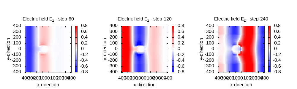
After we run the simulation, we can plot again the z-component of the electric
field in the xz-plane for three different time steps, using the following script:
gnuplot script
set pm3d
set view map
set palette defined ( -0.05 "blue" , 0 "white" , 0.05"red" )
set term png size 1000,300
unset surface
unset key
set output 'tutorial_04.1-drude-01.png'
set xlabel 'x-direction'
set ylabel 'y-direction'
set cbrange [ -0.8:0.8]
set multiplot
set origin 0.025,0
set size 0.3,0.9
set size square
set title 'Electric field E_z - step 60'
sp [ -400:400][ -400:400] 'Maxwell/output_iter/td.0000060/e_field-z.y=0' u ( $1 /18.897) :( $2 /18.897) :3
set origin 0.35,0
set size 0.3,0.9
set size square
set title 'Electric field E_z - step 120'
sp [ -400:400][ -400:400] 'Maxwell/output_iter/td.0000120/e_field-z.y=0' u ( $1 /18.897) :( $2 /18.897) :3
set origin 0.675,0
set size 0.3,0.9
set size square
set title 'Electric field E_z - step 240'
sp [ -400:400][ -400:400] 'Maxwell/output_iter/td.0000240/e_field-z.y=0' u ( $1 /18.897) :( $2 /18.897) :3
unset multiplot
The plot we get is the following:
As it is expected, as the medium reacts to the external field via its
polarization current density, screening it inside the sphere, as it is expected
from a metal. We can also note that the space discretization used is a rather
coarse mesh in this tutorial, due to computation time, but the outcomes are
still reasonable.
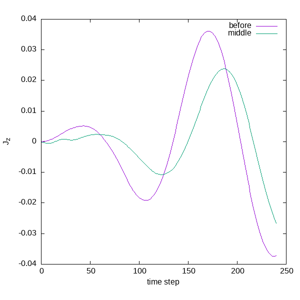
Finally, we can examine how these currents arise in time. Using the following
script we can plot the current at three different points (the ones we requested
in the input file, namely: near the surface of the sphere towards the negative
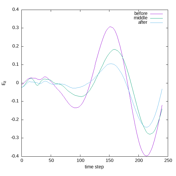
x axis, in the middle, and near the surface on the positive x axis). Also we
plot the E field at these points.
gnuplot script
set term png size 600,600
set output 'tutorial_04.1-drude-02.png'
set xlabel 'time step'
set ylabel 'J_z'
set size square
plot 'NP/td.general/current_at_points' u 1:5 w l title "before" , 'NP/td.general/current_at_points' u 1:8 w l title "middle" , 'NP/td.general/current_at_points' u 1:11 w l title "after"
set output 'tutorial_04.1-drude-03.png'
set xlabel 'time step'
set ylabel 'E_z'
set size square
plot 'Maxwell/td.general/total_e_field_z' u 1:3 w l title "before" , 'Maxwell/td.general/total_e_field_z' u 1:4 w l title "middle" , 'Maxwell/td.general/total_e_field_z' u 1:5 w l title "after"
As can be seen, the current in the direction of the incident electric field
(called “before”) is larger, screening the field effectively. This can be seen
by plotting the electric field in the other points, where the values in the
“middle” and “after” are much smaller than “before” (actually, the plotted
field has already been quenched by the medium, otherwise the waveform would be
that of the Gaussian envelope used). In addition to scattering, there is
absorption of energy by the nanoparticle, given by the imaginary part of the
polarizability. Using a setup like this, and processing the proper values of
the EM field in full space and time, it would be possible to calculate an
extinction spectrum of the sphere, which can be compared to the one calculated
using Mie theory, or other methods.
Prev
Next