Getting started with periodic systems
The extension of a ground-state calculation to a periodic system is quite straightforward in Octopus. In this tutorial we will explain how to perform some basic calculation using bulk silicon as an example.
Input
As always, we will start with a simple input file. In this case we will use a primitive cell of Si, composed of two atoms.
CalculationMode = gs

PeriodicDimensions = 3

Spacing = 0.5

a = 10.18
%LatticeParameters
 a | a | a
%

%LatticeVectors
 0.0 | 0.5 | 0.5
 0.5 | 0.0 | 0.5
 0.5 | 0.5 | 0.0
%

%ReducedCoordinates
 "Si" | 0.0 | 0.0 | 0.0
 "Si" | 1/4 | 1/4 | 1/4
%

nk = 2
%KPointsGrid
  nk |  nk |  nk
 0.5 | 0.5 | 0.5
 0.5 | 0.0 | 0.0
 0.0 | 0.5 | 0.0
 0.0 | 0.0 | 0.5
%
KPointsUseSymmetries = yes

Eigensolver = chebyshev_filter
ExtraStates = 4

%Output
 dos
%
Lets see more in detail some of the input variables:
-
PeriodicDimensions = 3: this input variable must be set equal to the number of dimensions you want to consider as periodic. Since the system is 3D (Dimensions = 3is the default), by setting this variable to 3 we impose periodic boundary conditions at all borders. This means that we have a fully periodic infinite crystal. -
LatticeVectorsandLatticeParameters: these two blocks are used to define the primitive lattice vectors that determine the unit cell.LatticeVectorsdefines the direction of the vectors, while LatticeParameters defines their length. -
ReducedCoordinates: the position of the atoms inside the unit cell, in reduced coordinates. -
KPointsGrid: this specifies the ‘‘k’’-point grid to be used in the calculation. Here we employ a 2x2x2 Monkhorst-Pack grid with four shifts. The first line of the block defines the number of ‘‘k’’-points along each axis in the Brillouin zone. Since we want the same number of points along each direction, we have defined the auxiliary variablenk = 2This will be useful later on to study the convergence with respect to the number of ‘‘k’’-points. The other four lines define the shifts, one per line, expressed in reduced coordinates of the Brillouin zone. Alternatively, one can also define the reciprocal-space mesh by explicitly setting the position and weight of each ‘‘k’’-point using the KPoints or KPointsReduced variables. -
KPointsUseSymmetries = yes: this variable controls if symmetries are used or not. When symmetries are used, the code shrinks the Brillouin zone to its irreducible portion and the effective number of ‘‘k’’-points is adjusted. -
Output = dos: we ask the code to output the density of states.
Here we have taken the value of the grid spacing to be 0.5 bohr. Although we will use this value throughout this tutorial, remember that in a real-life calculation the convergence with respect to the grid spacing must be performed for all quantities of interest.
Note that for periodic systems the default value for the BoxShape variable is parallelepiped, although in this case the name can be misleading, as the actual shape also depends on the lattice vectors. This is the only box shape currently available for periodic systems.
Output
Now run Octopus using the above input file. Here are some important things to note from the output.
******************************* Space ********************************
Octopus will run in 3 dimension(s).
Octopus will treat the system as periodic in 3 dimension(s).
**********************************************************************
******************************** Grid ********************************
Simulation Box:
  Type = parallelepiped
  Lengths [b] = (   7.198,   7.198,   7.198)
Main mesh:
  Spacing [b] = ( 0.514, 0.514, 0.514)    volume/point [b^3] =      0.09612
  # inner mesh =       2744
  # total mesh =       9192
  Grid Cutoff [H] =    18.666387    Grid Cutoff [Ry] =    37.332774
**********************************************************************
Here Octopus outputs some information about the cell in real and reciprocal space.
***************************** Symmetries *****************************
Space group No.  227
International: Fd-3m
Schoenflies: Oh^7
Info: The system has    24 symmorphic symmetries that can be used.
  Index                Rotation matrix                      Fractional translations
    1 :     1   0   0     0   1   0     0   0   1      0.000000    0.000000    0.000000
    2 :     0   1  -1     1   0  -1     0   0  -1      0.000000    0.000000    0.000000
    3 :    -1   0   0    -1   0   1    -1   1   0      0.000000    0.000000    0.000000
    4 :     0  -1   1     0  -1   0     1  -1   0      0.000000    0.000000    0.000000
    5 :     0   1   0     0   0   1     1   0   0      0.000000    0.000000    0.000000
    6 :    -1   0   1    -1   1   0    -1   0   0      0.000000    0.000000    0.000000
    7 :     0  -1   0     1  -1   0     0  -1   1      0.000000    0.000000    0.000000
    8 :     1   0  -1     0   0  -1     0   1  -1      0.000000    0.000000    0.000000
    9 :     0   0   1     1   0   0     0   1   0      0.000000    0.000000    0.000000
   10 :     1  -1   0     0  -1   1     0  -1   0      0.000000    0.000000    0.000000
   11 :     0   0  -1     0   1  -1     1   0  -1      0.000000    0.000000    0.000000
   12 :    -1   1   0    -1   0   0    -1   0   1      0.000000    0.000000    0.000000
   13 :    -1   0   1    -1   0   0    -1   1   0      0.000000    0.000000    0.000000
   14 :     0  -1   0     0  -1   1     1  -1   0      0.000000    0.000000    0.000000
   15 :     0   1   0     1   0   0     0   0   1      0.000000    0.000000    0.000000
   16 :     1   0  -1     0   1  -1     0   0  -1      0.000000    0.000000    0.000000
   17 :     1  -1   0     0  -1   0     0  -1   1      0.000000    0.000000    0.000000
   18 :     0   0  -1     1   0  -1     0   1  -1      0.000000    0.000000    0.000000
   19 :     0   0   1     0   1   0     1   0   0      0.000000    0.000000    0.000000
   20 :    -1   1   0    -1   0   1    -1   0   0      0.000000    0.000000    0.000000
   21 :     0   1  -1     0   0  -1     1   0  -1      0.000000    0.000000    0.000000
   22 :    -1   0   0    -1   1   0    -1   0   1      0.000000    0.000000    0.000000
   23 :     1   0   0     0   0   1     0   1   0      0.000000    0.000000    0.000000
   24 :     0  -1   1     1  -1   0     0  -1   0      0.000000    0.000000    0.000000
Info: The system also has    24 nonsymmorphic symmetries (not used for electrons).
    1 :     1   0  -1     1   0   0     1  -1   0      0.250000    0.250000    0.250000
    2 :     0   1   0     0   1  -1    -1   1   0      0.250000    0.250000    0.250000
    3 :     0  -1   0    -1   0   0     0   0  -1      0.250000    0.250000    0.250000
    4 :    -1   0   1     0  -1   1     0   0   1      0.250000    0.250000    0.250000
    5 :    -1   1   0     0   1   0     0   1  -1      0.250000    0.250000    0.250000
    6 :     0   0   1    -1   0   1     0  -1   1      0.250000    0.250000    0.250000
    7 :     0   0  -1     0  -1   0    -1   0   0      0.250000    0.250000    0.250000
    8 :     1  -1   0     1   0  -1     1   0   0      0.250000    0.250000    0.250000
    9 :     0  -1   1     0   0   1    -1   0   1      0.250000    0.250000    0.250000
   10 :     1   0   0     1  -1   0     1   0  -1      0.250000    0.250000    0.250000
   11 :    -1   0   0     0   0  -1     0  -1   0      0.250000    0.250000    0.250000
   12 :     0   1  -1    -1   1   0     0   1   0      0.250000    0.250000    0.250000
   13 :    -1   0   0     0  -1   0     0   0  -1      0.250000    0.250000    0.250000
   14 :     0  -1   1    -1   0   1     0   0   1      0.250000    0.250000    0.250000
   15 :     1   0   0     1   0  -1     1  -1   0      0.250000    0.250000    0.250000
   16 :     0   1  -1     0   1   0    -1   1   0      0.250000    0.250000    0.250000
   17 :     0  -1   0     0   0  -1    -1   0   0      0.250000    0.250000    0.250000
   18 :     1   0  -1     1  -1   0     1   0   0      0.250000    0.250000    0.250000
   19 :     0   1   0    -1   1   0     0   1  -1      0.250000    0.250000    0.250000
   20 :    -1   0   1     0   0   1     0  -1   1      0.250000    0.250000    0.250000
   21 :     0   0  -1    -1   0   0     0  -1   0      0.250000    0.250000    0.250000
   22 :    -1   1   0     0   1  -1     0   1   0      0.250000    0.250000    0.250000
   23 :     0   0   1     0  -1   1    -1   0   1      0.250000    0.250000    0.250000
   24 :     1  -1   0     1   0   0     1   0  -1      0.250000    0.250000    0.250000
**********************************************************************
This block tells us about the space-group and the symmetries found for the specified structure. Note that Octopus can identify so-called non-symmorphic symmetry operation, but these are not used to symmetrize the density.
****************************** Lattice *******************************
  Lattice Vectors [b]
    0.000000    5.090000    5.090000
    5.090000    0.000000    5.090000
    5.090000    5.090000    0.000000
  Cell volume =           263.7445 [b^3]
  Reciprocal-Lattice Vectors [b^-1]
   -0.617209    0.617209    0.617209
    0.617209   -0.617209    0.617209
    0.617209    0.617209   -0.617209
  Cell angles [degree]
    alpha =   60.000
    beta  =   60.000
    gamma =   60.000
**********************************************************************
Checking if the generated full k-point grid is symmetric

     2 k-points generated from parameters :
 ---------------------------------------------------
    n =    2    2    2

    s1  =  0.50  0.50  0.50

    s2  =  0.50  0.00  0.00

    s3  =  0.00  0.50  0.00

    s4  =  0.00  0.00  0.50

   index |      weight  |             coordinates              |
       1 |     0.250000 |    0.250000    0.000000    0.000000  |
       2 |     0.750000 |   -0.250000    0.250000    0.250000  |
Next we get the list of the ‘‘k’’-points in reduced coordinates and their weights. Since symmetries are used, only two ‘‘k’’-points are generated. If we had not used symmetries, we would have 32 ‘‘k’’-points instead.
The rest of the output is much like its non-periodic counterpart. After a few iterations the code should converge:
*********************** SCF CYCLE ITER #   10 ************************
 etot  = -7.92930513E+00 abs_ev   =  5.87E-07 rel_ev   =  2.38E-06
 ediff =        7.63E-07 abs_dens =  9.08E-07 rel_dens =  1.14E-07
Matrix vector products:     50
Converged eigenvectors:      0

#  State  KPoint  Eigenvalue [H]  Occupation    Error
      1       1       -0.257166    2.000000   ( 1.5E-07)
      1       2       -0.184854    2.000000   ( 1.4E-07)
      2       2       -0.079338    2.000000   ( 1.4E-07)
      2       1        0.010755    2.000000   ( 1.6E-07)
      3       2        0.023126    2.000000   ( 1.5E-07)
      4       2        0.073568    2.000000   ( 1.7E-07)
      3       1        0.127870    2.000000   ( 2.0E-07)
      4       1        0.127870    2.000000   ( 2.0E-07)
      5       2        0.208837    0.000000   ( 9.1E-08)
      5       1        0.231967    0.000000   ( 1.5E-07)
      6       1        0.284821    0.000000   ( 2.5E-07)
      7       1        0.284821    0.000000   ( 2.5E-07)
      6       2        0.317717    0.000000   ( 1.5E-05)
      7       2        0.368948    0.000000   ( 2.0E-03)
      8       2        0.374076    0.000000   ( 4.8E-03)
      8       1        0.412807    0.000000   ( 1.0E-01)

Density of states:

-------%----------%----------%----%-------------%----------%----%%----
-------%----------%----------%----%-------------%----------%----%%----
-------%----------%----------%----%-------------%----------%----%%----
-------%----------%----------%----%-----%-------%-------%--%----%%----
-------%----------%----------%----%-----%-------%-------%--%----%%----
-------%----------%----------%----%-----%-------%-------%--%----%%----
-------%----------%----------%----%-----%-------%-------%--%----%%----
%------%----------%---------%%----%-----%-------%-%-----%--%----%%---%
%------%----------%---------%%----%-----%-------%-%-----%--%----%%---%
%------%----------%---------%%----%-----%-------%-%-----%--%----%%---%
                                        ^


Elapsed time for SCF step    10:          0.01
**********************************************************************

             Info: Writing states. 2025/04/03 at 22:58:42


        Info: Finished writing states. 2025/04/03 at 22:58:42

Info: SCF converged in   10 iterations

Info: Number of matrix-vector products:        500
Info: Writing output to static/
Info: Finished writing information to 'restart/gs'.

             Calculation ended on 2025/04/03 at 22:58:42

                          Walltime:  00.788s

Octopus emitted 14 warnings.
As usual, the static/info file contains the most relevant information concerning the calculation. Since we asked the code to output the density of states, we also have a few new files in the static directory:
- dos-XXXX.dat : the band-resolved density of states (DOS);
- total-dos.dat : the total DOS (summed over all bands);
- total-dos-efermi.dat : the Fermi Energy in a format compatible with total-dos.dat .
Of course you can tune the output type and format in the same way you do in a finite-system calculation.
Convergence in k-points
Similar to the convergence in spacing, a convergence must be performed for the sampling of the Brillouin zone. To do this one must try different numbers of ‘‘k’’-points along each axis in the Brillouin zone. This can easily be done by changing the value of the nk auxiliary variable in the previous input file. You can obviously do this by hand, but this is something that can also be done with a script. Here is such a script, which we will name kpts.sh :
#!/bin/bash
echo "#nk Total Energy" > kpts.dat
list="2 4 6 8 10 12"
for nkpt in $list
do
    echo "$nkpt"
    sed -i "s/nk = [0-9]\+/nk = $nkpt/" inp
    octopus >& out-$nkpt
    energy=`grep Total static/info  | head -2 | tail -1 | cut -d "=" -f 2`
    echo $nkpt $energy >> kpts.dat
    rm -rf restart
done
After running the script (source kpts.sh), you should obtain a file called kpts.dat
that should look like this:
#nk Total Energy
2 -7.92930513
4 -7.93539038
6 -7.93548819
8 -7.93549116
10 -7.93549133
12 -7.93549133
As you can see, the total energy is converged to within 0.0001 Hartree for nk = 6.
You can now play with an extended range, e.g. from 2 to 12. You should then see that the total energy is converged to less than a micro Hartree.
Band-structure
We now proceed with the calculation of the band-structure of Si. In order to compute a band-structure, we must perform a non-self-consistent calculation, using the density of a previous ground-state calculation. So the first step is to obtain the initial ground-state. To do this, rerun the previous input file, but changing the number of k-points to nk=6. Next, modify the input file such that it looks like this:
CalculationMode = unocc

PeriodicDimensions = 3

Spacing = 0.5

a = 10.18
%LatticeParameters
 a | a | a
%

%LatticeVectors
 0.0 | 0.5 | 0.5
 0.5 | 0.0 | 0.5
 0.5 | 0.5 | 0.0
%

%ReducedCoordinates
 "Si" | 0.0 | 0.0 | 0.0
 "Si" | 1/4 | 1/4 | 1/4
%

Eigensolver = chebyshev_filter

ExtraStates = 10
ExtraStatesToConverge = 5

%KPointsPath
  10 |  10 |  15
 0.5 | 0.0 | 0.0  # L point
 0.0 | 0.0 | 0.0  # Gamma point
 0.0 | 0.5 | 0.5  # X point
 1.0 | 1.0 | 1.0  # Another Gamma point
%
KPointsUseSymmetries = no
Here are the things we changed:
-
CalculationMode = unocc: we are now performing a non-self-consistent calculation, so we use theunoccupiedcalculation mode; -
ExtraStates = 10: this is the number of unoccupied bands to calculate; -
ExtraStatesToConverge = 5: the highest unoccupied states are very hard to converge, so we use this variable to specify how many unoccupied states are considered for the stopping criterion of the non-self-consistent run. -
KPointsPath: this block is used to specify that we want to calculate the band structure along a certain path in the Brillouin zone. This replaces the KPointsGrid block. The first row describes how many ‘‘k’’-points will be used to sample each segment. The next rows are the coordinates of the ‘‘k’’-points from which each segment starts and stops. In this particular example, we chose the following path: L-Gamma, Gamma-X, X-Gamma using a sampling of 10-10-15 ‘‘k’’-points. -
KPointsUseSymmetries = no: we have turned off the use of symmetries.
After running Octopus with this input file, you should obtain a file named bandstructure inside the static directory. This is how the first few lines of the file should look like:
# coord. kx ky kz (red. coord.), bands:    14 [H]
     0.00000000    0.50000000    0.00000000    0.00000000    -0.19991863    -0.10472287     0.11047036     0.11047036     0.21305881     0.27686198     0.27686198     0.43507023     0.54432356     0.54432356     0.57081122     0.57480604     0.57480604     0.63375689
     0.02640129    0.45000000   -0.00000000   -0.00000000    -0.20513536    -0.09720635     0.11112992     0.11112992     0.21381242     0.27766711     0.27766711     0.43630357     0.51921716     0.51921716     0.55502890     0.60261190     0.60261190     0.64782332
     0.05280258    0.40000000   -0.00000000   -0.00000000    -0.21732506    -0.07814040     0.11310636     0.11310636     0.21606165     0.27985733     0.27985733     0.43957700     0.48667806     0.48667806     0.52605166     0.64299566     0.64299567     0.66836316
     0.07920387    0.35000000    0.00000000    0.00000000    -0.23165576    -0.05243052     0.11638749     0.11638749     0.21976491     0.28269162     0.28269162     0.44256490     0.45780277     0.45780277     0.49752185     0.66341823     0.68308997     0.68321622
...
The first column is the coordinate of the ‘‘k’’-point along the path. The second, third, and fourth columns are the reduced coordinates of the ‘‘k’’-point. The following columns are the eigenvalues for the different bands. In this case there are 14 bands (4 occupied and 10 unoccupied).
Below you can see the plot of the band structure.
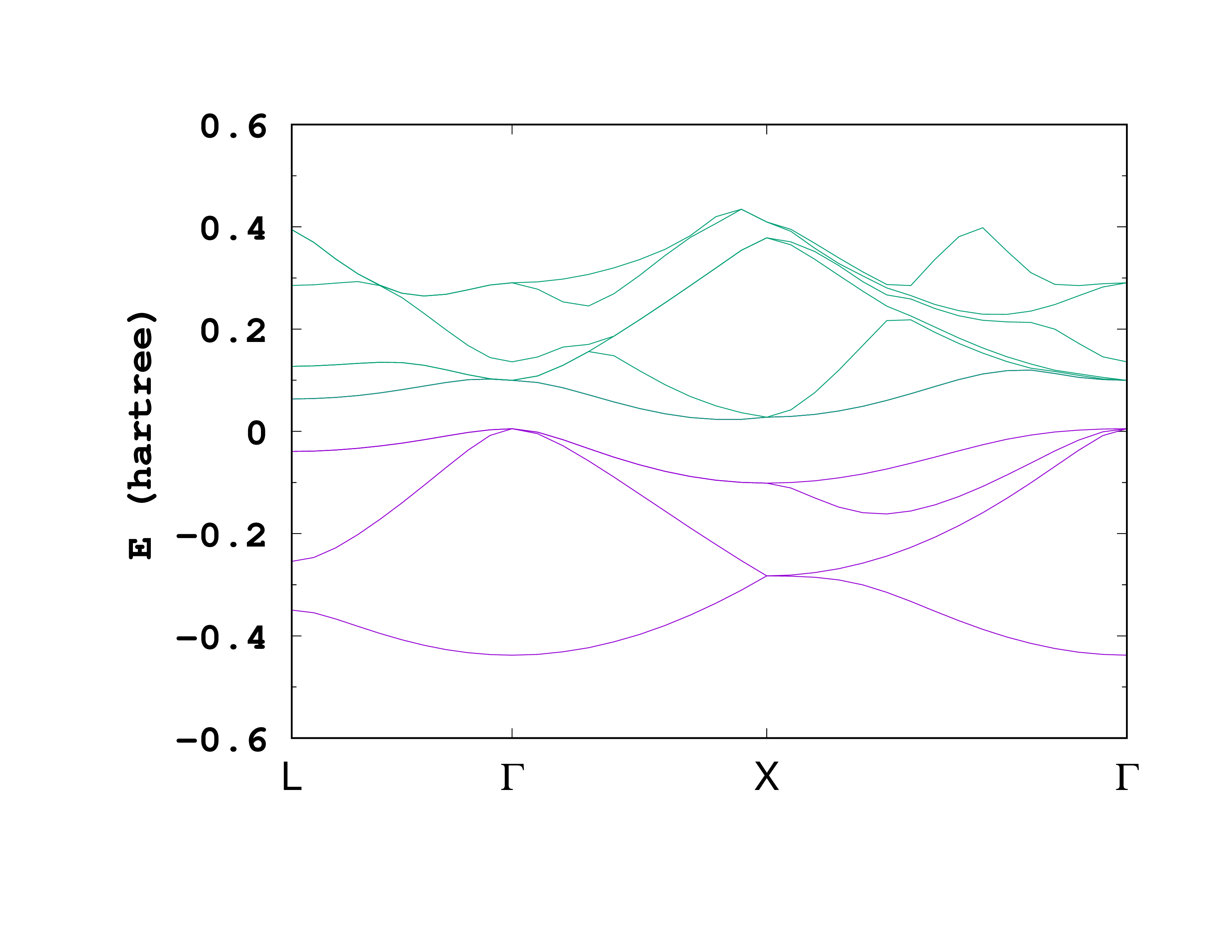
This plot shows the occupied bands (purple) and the first 5 unoccupied bands (green). If you are using gnuplot, you can obtain a similar plot with the following command:
plot for [col=5:5+9] 'static/bandstructure' u 1:(column(col)) w l notitle ls 1
Note that when using the KPointsPath input variable, Octopus will run in a special mode, which has some effects on the restart system: As we are using different k-points, as used in the ground state calculation, the code issues warnings about incompatible restart information. Furthermore, the restart information of the previous ground-state calculation will not be altered in any way. The code informs us about this just before starting the unoccupied states iterations:
Info: The code will run in band structure mode.
     No restart information will be printed.