Geometry optimization
In this tutorial we will show how to perform geometry optimizations using Octopus.
Methane molecule
Manual optimization
We will start with the methane molecule. Before using any sophisticated algorithm for the geometry optimization, it is quite instructive to do it first “by hand”. Of course, this is only practical for systems with very few degrees of freedom, but this is the case for methane, as we only need to optimize the CH bond-length. We will use the following files.
inp file
CalculationMode = gs
UnitsOutput = eV_Angstrom

Radius = 3.5*angstrom
Spacing = 0.18*angstrom

CH = 1.30*angstrom
%Coordinates
  "C" |           0 |          0 |           0
  "H" |  CH/sqrt(3) | CH/sqrt(3) |  CH/sqrt(3)
  "H" | -CH/sqrt(3) |-CH/sqrt(3) |  CH/sqrt(3)
  "H" |  CH/sqrt(3) |-CH/sqrt(3) | -CH/sqrt(3)
  "H" | -CH/sqrt(3) | CH/sqrt(3) | -CH/sqrt(3)
%
This input file is similar to ones used in other tutorials. We have seen in the Total_energy_convergence tutorial that for these values of the spacing and radius the total energy was converged to within 0.1 eV.
ch.sh script
You can run the code by hand, changing the bond-length for each calculation, but you can also use the following script:
#!/bin/bash
echo "#CH distance   Total Energy" > ch.dat
list="0.90 0.95 1.00 1.05 1.10 1.15 1.20 1.25 1.30"
for CH in $list
do
    echo $CH
    sed -ie "/CH = /s|[0-9.]\+|$CH|" inp
    mpirun -n 4 octopus >& out-$CH
    energy=`grep Total static/info  | head -1 | cut -d "=" -f 2`
    echo $CH $energy >> ch.dat
    rm -rf restart
done
Results
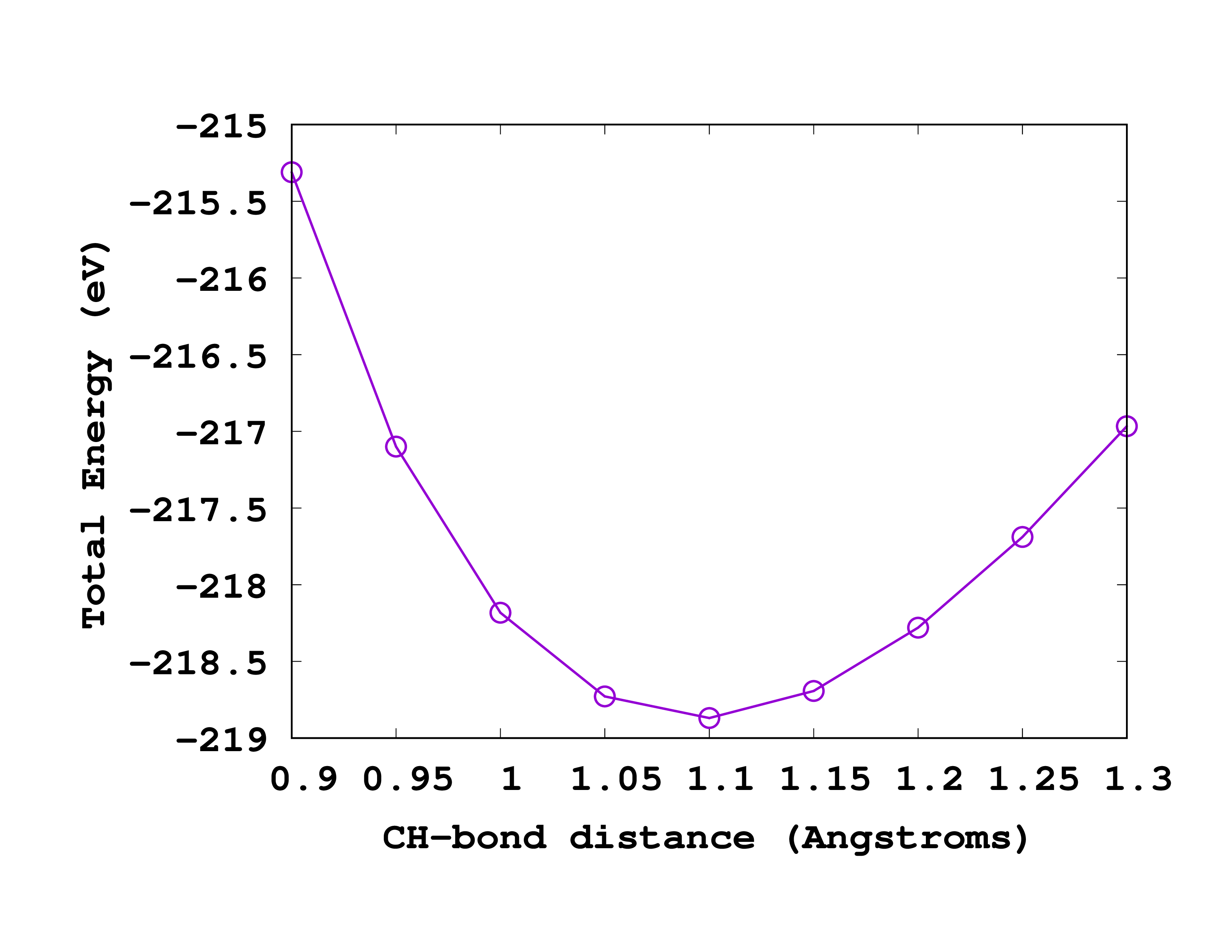
Once you run the calculations, you should obtain values very similar to the following ones:
#CH distance   Total Energy
0.90 -215.31079467
0.95 -217.09923522
1.00 -218.18219528
1.05 -218.72869220
1.10 -218.86934526
1.15 -218.69291939
1.20 -218.27943421
1.25 -217.68882326
1.30 -216.96631252
You can see on the right how this curve looks like when plotted. By simple inspection we realize that the equilibrium CH distance that we obtain is around 1.1 Å. This should be compared to the experimental value of 1.094 Å. From this data can you calculate the frequency of the vibrational breathing mode of methane?
FIRE
Since changing the bond-lengths by hand is not exactly the simplest method to perform the geometry optimization, we will now use automated algorithms for doing precisely that. Several of these algorithms are available in Octopus. The default and recommend one is the the FIRE method1 . Octopus can also use the GSL optimization routines, so all the methods provided by this library are available.
Input
First we will run a simple geometry optimization using the following input file:
FromScratch = yes
CalculationMode = go
UnitsOutput = eV_Angstrom

GOMethod = fire

BoxShape = sphere
Radius = 5*angstrom
Spacing = 0.18*angstrom

CH = 1.2*angstrom
%Coordinates
  "C" |           0 |          0 |           0
  "H" |  CH/sqrt(3) | CH/sqrt(3) |  CH/sqrt(3)
  "H" | -CH/sqrt(3) |-CH/sqrt(3) |  CH/sqrt(3)
  "H" |  CH/sqrt(3) |-CH/sqrt(3) | -CH/sqrt(3)
  "H" | -CH/sqrt(3) | CH/sqrt(3) | -CH/sqrt(3)
%
In this case we are using default values for all the input variables related to the geometry optimization. Compared to the input file above, we have changed the CalculationMode to go. Because the default minimum box of spheres centered on the atoms has some caveats when performing a geometry optimization (see bellow for more details), we also changed the box shape to a single sphere with a 5 Å radius. Like always, convergence of the final results should be checked with respect to the mesh parameters. In this case you can trust us that a radius of 5 Å is sufficient.
The geometry in the input file will be used as a starting point. Note that although a single variable CH was used to specify the structure, the coordinates will be optimized independently.
Output
When running Octopus in geometry optimization mode the output will be a bit different from the normal ground-state mode. Since each minimization step requires several SCF cycles, only one line of information for each SCF iteration will printed:
Info: Starting SCF iteration.
iter    1 : etot -2.27991992E+02 : abs_dens 2.03E+00 : etime     0.7s
iter    2 : etot -2.27947938E+02 : abs_dens 1.81E-01 : etime     0.1s
iter    3 : etot -2.21131250E+02 : abs_dens 4.01E-01 : etime     0.4s
iter    4 : etot -2.17934989E+02 : abs_dens 2.16E-01 : etime     0.2s
iter    5 : etot -2.18667820E+02 : abs_dens 6.44E-02 : etime     0.2s
iter    6 : etot -2.18394307E+02 : abs_dens 1.23E-02 : etime     0.2s
iter    7 : etot -2.18301945E+02 : abs_dens 2.80E-03 : etime     0.3s
iter    8 : etot -2.18295247E+02 : abs_dens 2.24E-04 : etime     0.2s
iter    9 : etot -2.18290443E+02 : abs_dens 1.19E-04 : etime     0.1s
iter   10 : etot -2.18286567E+02 : abs_dens 1.00E-04 : etime     0.2s
iter   11 : etot -2.18286878E+02 : abs_dens 8.22E-06 : etime     0.1s
iter   12 : etot -2.18286749E+02 : abs_dens 8.95E-06 : etime     0.2s
iter   13 : etot -2.18286927E+02 : abs_dens 2.06E-06 : etime     0.1s
iter   14 : etot -2.18286925E+02 : abs_dens 8.01E-07 : etime     0.1s

             Info: Writing states. 2024/10/18 at 10:41:24


        Info: Finished writing states. 2024/10/18 at 10:41:24

Info: SCF converged in   14 iterations

Info: Number of matrix-vector products:        350
Info: Starting SCF iteration.
At the end of each minimization step the code will print the total energy, the maximum force acting on the ions and the maximum displacement of the ions from the previous geometry to the next one. Octopus will also print the current geometry to a file named go.XXXX.xyz (XXXX is the minimization iteration number) in a directory named geom . In the working directory there is also a file named work-geom.xyz that accumulates the geometries of each SCF calculation. The results are also summarized in geom/optimization.log . The most recent individual geometry is in last.xyz .
After some minimization steps the code will exit.
++++++++++++++++++++++++++++++++++++++++++++++++++++++++++++++++++++++
+++++++++++++++++++++ MINIMIZATION ITER #:   31 ++++++++++++++++++++++
  Energy    = -218.8768110116 eV
  Max force =    0.0349131063 eV/A
  Max dr    =    0.0010886077 A
++++++++++++++++++++++++++++++++++++++++++++++++++++++++++++++++++++++
++++++++++++++++++++++++++++++++++++++++++++++++++++++++++++++++++++++


Writing final coordinates to min.xyz
Info: Finished writing information to 'restart/gs'.
If the minimization was successful a file named min.xyz will be written in the working directory containing the minimized geometry. In this case it should look like this:
   5
 units: A
      C                   -0.000000    0.000000    0.000000
      H                    0.631869    0.631869    0.631869
      H                   -0.631869   -0.631869    0.631869
      H                    0.631869   -0.631869   -0.631869
      H                   -0.631869    0.631869   -0.631869
Has the symmetry been retained? What is the equilibrium bond length determined? Check the forces in static/info . You can also visualize the optimization process as an animation by loading work-geom.xyz as an XYZ file into XCrySDen.
Sodium trimer
Let’s now try something different: a small sodium cluster. This time we will use an alternate method related to conjugate gradients.
Input
Here is the input file to use
FromScratch = yes
CalculationMode = go
UnitsOutput = eV_Angstrom

radius = 6.0*angstrom
spacing = 0.3*angstrom

XYZCoordinates = "inp.xyz"

GOMethod = cg_bfgs
and the corresponding inp.xyz file
  3

  Na     -1.65104552837    -1.51912734276    -1.77061890357
  Na     -0.17818042320    -0.81880768425    -2.09945089196
  Na      1.36469690888     0.914070162416    0.40877139068
In this case the starting geometry is a random geometry.
Output
After some time the code should stop successfully. The information about the last minimization iteration should look like this:
++++++++++++++++++++++++++++++++++++++++++++++++++++++++++++++++++++++
+++++++++++++++++++++ MINIMIZATION ITER #:    3 ++++++++++++++++++++++
  Energy    =  -16.8821035602 eV
  Max force =    0.0283223142 eV/A
  Max dr    =    0.1308932156 A
++++++++++++++++++++++++++++++++++++++++++++++++++++++++++++++++++++++
++++++++++++++++++++++++++++++++++++++++++++++++++++++++++++++++++++++


Writing final coordinates to min.xyz
Info: Finished writing information to 'restart/gs'.
You might have noticed that in this case the code might perform several SCF cycles for each minimization iteration. This is normal, as the minimization algorithm used here requires the evaluation of the energy and forces at several geometries per minimization iteration. The minimized geometry can be found in the min.xyz file:
  3

  Na     -1.65104552837    -1.51912734276    -1.77061890357
  Na     -0.17818042320    -0.81880768425    -2.09945089196
  Na      1.36469690888     0.914070162416    0.40877139068
Caveats of using a minimum box
For this example we are using the minimum box (BoxShape = minimum). This box shape is the one used by default, as it is usually the most efficient one, but it requires some care when using it for a geometry optimization. The reason is that the box is generated at the beginning of the calculation and is not updated when the atoms move. This means that at the end of the optimization, the centers of the spheres composing the box will not coincide anymore with the position of the atoms. This is a problem if the atoms move enough such that their initial and final positions differ significantly. If this is the case, the best is to restart the calculation using the previously minimized geometry as the starting geometry, so that the box is constructed again consistently with the atoms. In this example, this can be done by copying the contents of the min.xyz
file inp.xyz
and running Octopus again without changing input file.
This time the calculation should converge after only one iteration:
++++++++++++++++++++++++++++++++++++++++++++++++++++++++++++++++++++++
+++++++++++++++++++++ MINIMIZATION ITER #:    1 ++++++++++++++++++++++
  Energy    =  -16.8903481568 eV
  Max force =    0.0409500446 eV/A
  Max dr    =    0.0423429600 A
++++++++++++++++++++++++++++++++++++++++++++++++++++++++++++++++++++++
++++++++++++++++++++++++++++++++++++++++++++++++++++++++++++++++++++++


Writing final coordinates to min.xyz
Info: Finished writing information to 'restart/gs'.
You can now compare the old min.xyz file with the new one:
   3
 units: A
      Na                  -2.267804   -1.807298   -1.618175
      Na                   0.456021   -0.515796   -2.237107
      Na                   1.347075    0.899186    0.394174
Although the differences are not too large, there are also not negligible.
Further improving the geometry
Imagine that you now want to improve the geometry obtained and reduce the value of the forces acting on the ions. The stopping criterion is controlled by the GOTolerance variable (and GOMinimumMove). Its default value is 0.051 eV/Å (0.001 H/b), so let’s set it to 0.01 eV/Å:
FromScratch = yes
CalculationMode = go
UnitsOutput = eV_Angstrom

radius = 6.0*angstrom
spacing = 0.3*angstrom

XYZCoordinates = "inp.xyz"

GOMethod = cg_bfgs
GOTolerance = 0.01*eV/angstrom
Copy the contents of file min.xyz to file inp.xyz and rerun the code. This time, after some minimization steps Octopus should return the following error message:
 **************************** FATAL ERROR *****************************
 *** Fatal Error (description follows)
 *--------------------------------------------------------------------
 * Error occurred during the GSL minimization procedure:
 * iteration is not making progress towards solution
 **********************************************************************
This means the minimization algorithm was unable to improve the solutions up to the desired accuracy. Unfortunately there are not many things that can be done in this case. The most simple one is just to restart the calculation starting from the last geometry (use the last go.XXXX.xyz file) and see if the code is able to improve further the geometry.
-
Erik Bitzek, Pekka Koskinen, Franz Gähler, Michael Moseler, and Peter Gumbsch, Structural relaxation made simple, Phys. Rev. Lett. 97 170201 (2006); ↩︎