Plane waves in vacuum
Cosinoidal plane wave in vacuum
In this tutorial, we will describe the propagation of waves in vacuum. Let’s start with one wave with a cosinoidal envelope.
# ----- Calculation mode and parallelization ------------------------------------------------------

 CalculationMode   = td
 RestartWrite = no
 ExperimentalFeatures = yes
 FromScratch = yes

%Systems
  'Maxwell' | maxwell
%

 Maxwell.ParDomains = auto
 Maxwell.ParStates  = no

# ----- Maxwell box variables ---------------------------------------------------------------------

 # free maxwell box limit of 10.0 plus 2.0 for the incident wave boundaries with
 # der_order = 4 times dx_mx

 lsize_mx = 12.0
 dx_mx         = 0.5 0.85

 Maxwell.BoxShape   = parallelepiped

 %Maxwell.Lsize
  lsize_mx | lsize_mx | lsize_mx
 %

 %Maxwell.Spacing
  dx_mx | dx_mx | dx_mx
 %


# ----- Maxwell calculation variables -------------------------------------------------------------

 MaxwellHamiltonianOperator = faraday_ampere

 %MaxwellBoundaryConditions
  plane_waves | plane_waves | plane_waves
 %

 %MaxwellAbsorbingBoundaries
  not_absorbing | not_absorbing | not_absorbing
 %

# ----- Output variables --------------------------------------------------------------------------

 OutputFormat = plane_x + plane_y + plane_z + vtk + axis_x

# ----- Maxwell output variables ------------------------------------------------------------------

 %MaxwellOutput
  electric_field
  magnetic_field
  maxwell_energy_density
  poynting_vector | plane_z
  orbital_angular_momentum | plane_z
 %

 %MaxwellFieldsCoordinate
   0.00 | 0.00 | 0.00
   0.00 | 0.00 | -5.00
   0.00 | 0.00 | 5.00
 %

 MaxwellOutputInterval = 50
 MaxwellTDOutput       = maxwell_energy + maxwell_total_e_field + maxwell_total_b_field + maxwell_transverse_e_field + maxwell_transverse_b_field


# ----- Time step variables -----------------------------------------------------------------------

 TDSystemPropagator = prop_expmid
 TDTimeStep                        = 0.002
 TDPropagationTime                 = 0.35

# ----- Maxwell field variables -------------------------------------------------------------------

 lambda = 10.0
 omega  = 2 * pi * c / lambda
 kx     = omega / c
 Ez     = 0.05
 pw     = 10.0
 p_s     = - 5 * 5.0

 %MaxwellIncidentWaves
   plane_wave_mx_function | electric_field | 0 | 0 | Ez | "plane_waves_function"
 %

 %MaxwellFunctions
   "plane_waves_function" | mxf_cosinoidal_wave | kx | 0 | 0 | p_s | 0 | 0 | pw
 %
The total size of the (physical) simulation box is 20.0 x 20.0 x 20.0 Bohr (10 Bohr half length in each direction) with a spacing of 0.5 Bohr in each direction. As discussed in the input overview, also the boundary points have to be accounted for when defining the box size in the input file. In other words, the user has to know how much space these points will add, which is given by the derivatives order (in this case, 4) times the spacing. This is 4 * 0.5 bohr = 2 bohr. Hence the total size of the simulation box is chosen to be 12.0 bohr in each direction.
# ----- Maxwell box variables ---------------------------------------------------------------------

 # free maxwell box limit of 10.0 plus 2.0 for the incident wave boundaries with
 # der_order = 4 times dx_mx

 lsize_mx = 12.0
 dx_mx         = 0.5 0.85

 Maxwell.BoxShape   = parallelepiped

 %Maxwell.Lsize
  lsize_mx | lsize_mx | lsize_mx
 %

 %Maxwell.Spacing
  dx_mx | dx_mx | dx_mx
 %
The boundary conditions are chosen as plane waves to simulate the incoming wave without any absorption at the boundaries.
 %MaxwellBoundaryConditions
  plane_waves | plane_waves | plane_waves
 %

 %MaxwellAbsorbingBoundaries
  not_absorbing | not_absorbing | not_absorbing
 %
The simulation time step is set to the value given by the Courant condition.
For equal spacing in the three dimensions, this is equal to dt = spacing /
(sqrt(3)*c) = 0.002106 atomic units of time, in this case,
c being the speed of light in atomic units (137.03599).
The system propagates 150 time steps = 0.316 atomic units.
# ----- Time step variables -----------------------------------------------------------------------

 TDSystemPropagator = prop_expmid
 TDTimeStep                        = 0.002
 TDPropagationTime                 = 0.35
The incident cosinoidal plane is evaluated at the boundaries to be fed into the simulation box. The pulse has a width of 10.0 bohr, a spatial shift of 25.0 Bohr in the negative x-direction, an amplitude of 0.05 a.u., and a wavelength of 10.0 bohr.
# ----- Maxwell field variables -------------------------------------------------------------------

 lambda = 10.0
 omega  = 2 * pi * c / lambda
 kx     = omega / c
 Ez     = 0.05
 pw     = 10.0
 p_s     = - 5 * 5.0

 %MaxwellIncidentWaves
   plane_wave_mx_function | electric_field | 0 | 0 | Ez | "plane_waves_function"
 %

 %MaxwellFunctions
   "plane_waves_function" | mxf_cosinoidal_wave | kx | 0 | 0 | p_s | 0 | 0 | pw
 %
Finally, the output options are set:
# ----- Output variables --------------------------------------------------------------------------

 OutputFormat = plane_x + plane_y + plane_z + vtk + axis_x

# ----- Maxwell output variables ------------------------------------------------------------------

 %MaxwellOutput
  electric_field
  magnetic_field
  maxwell_energy_density
  poynting_vector | plane_z
  orbital_angular_momentum | plane_z
 %

 %MaxwellFieldsCoordinate
   0.00 | 0.00 | 0.00
   0.00 | 0.00 | -5.00
   0.00 | 0.00 | 5.00
 %

 MaxwellOutputInterval = 50
 MaxwellTDOutput       = maxwell_energy + maxwell_total_e_field + maxwell_total_b_field + maxwell_transverse_e_field + maxwell_transverse_b_field
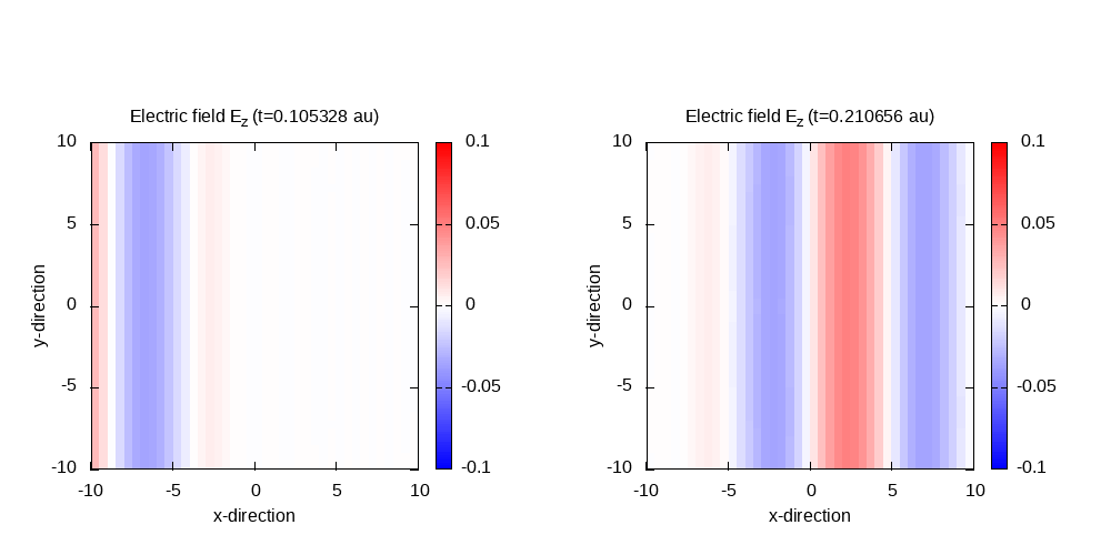
Contour plot of the electric field in z-direction after 50 time steps (t=0.105) and 100 time steps (t=0.21):
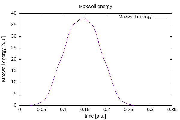
Maxwell energy inside the free Maxwell propagation region of the simulation box:
Interference of two cosinoidal plane waves
Instead of only one plane wave, we simulate in this example two different plane waves with different wave-vectors entering the simulation box, interfering and leaving the box again. In addition to the wave from the last tutorial, we add a second wave with different wave length, and entering the box at an angle, and shifted by 28 bohr along the corresponding direction of propagation. Both electric fields are polarized only in z-direction, and the magnetic field only in y-direction.
CalculationMode                   = td
ExperimentalFeatures = yes
FromScratch = yes

%Systems
  'Maxwell' | maxwell
%

Maxwell.ParStates                 = no

# Maxwell box variables
lsize_mx = 10.0

Maxwell.BoxShape                   = parallelepiped

%Maxwell.Lsize
 lsize_mx | lsize_mx | lsize_mx
%

dx_mx         = 0.5 0.85

%Maxwell.Spacing
 dx_mx | dx_mx | dx_mx
%

# Maxwell calculation variables
%MaxwellBoundaryConditions
 plane_waves | plane_waves | plane_waves
%

%MaxwellAbsorbingBoundaries
 not_absorbing | not_absorbing | not_absorbing
%

# Output variables
OutputFormat                      = axis_x + axis_y + axis_z + plane_z

# Maxwell output variables
%MaxwellOutput
 electric_field
 magnetic_field
 maxwell_energy_density
 trans_electric_field
%
MaxwellOutputInterval             = 10
MaxwellTDOutput                   = maxwell_energy

# Time step variables
TDSystemPropagator = prop_expmid
td = 1 / ( sqrt(c^2/dx_mx^2 + c^2/dx_mx^2 + c^2/dx_mx^2) )
TDTimeStep                        = td
TDPropagationTime                 = 0.35

# laser propagates in x direction
k_1_x       =  0.707107
k_1_y       = -0.707107
k_2_x       = -0.447214
k_2_y       = -0.223607
E_1_z       =  0.5
E_2_z       =  0.5
pw_1        =  5.0
pw_2        =  7.5
ps_1_x      = -sqrt(1/2) * 20.0
ps_1_y      =  sqrt(1/2) * 20.0
ps_2_x      =  sqrt(2/3) * 20.0
ps_2_y      =  sqrt(1/3) * 20.0

%MaxwellIncidentWaves
  plane_wave_mx_function | electric_field | 0 | 0 | E_1_z | "plane_waves_function_1"
  plane_wave_mx_function | electric_field | 0 | 0 | E_2_z | "plane_waves_function_2"
%

%MaxwellFunctions
  "plane_waves_function_1" | mxf_cosinoidal_wave | k_1_x | k_1_y | 0 | ps_1_x | ps_1_y | 0 | pw_1
  "plane_waves_function_2" | mxf_cosinoidal_wave | k_2_x | k_2_y | 0 | ps_2_x | ps_2_y | 0 | pw_2
%
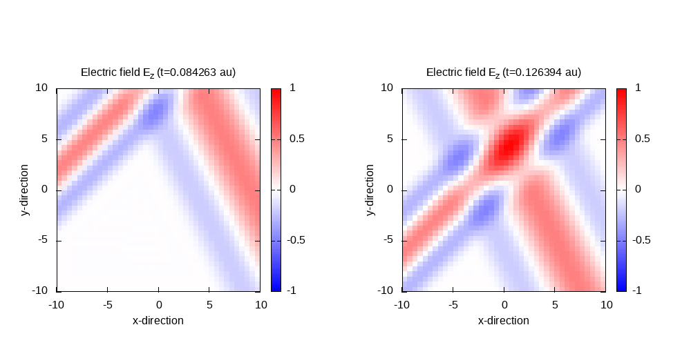
Using a similar script than in the previous example, the contour plots for the electric field in the z=0 plane can be obtained.
Contour plot of the electric field in z-direction after 40 time steps and 60 time steps:
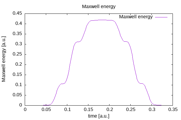
Total energy inside the propagation region of the simulation box: