All-electron calculations

Under certain conditions, it is possible to perform all-electron calculations in the Octopus code. In this tutorial, we explore how to perform an all-electron calculation for a carbon atom.

Here is the minimal input file needed to perform the calculation

%Coordinates
 'C_f' | 0 | 0 | 0
%

%Species
 'C_f' | species_full_delta | valence | 6
%

BoxShape = sphere
Radius = 9.0
Spacing = 0.2

ExtraStates = 2

%Occupations
 2/3 | 2/3 | 2/3
%

We employed here a species type called “species_full_delta”. The idea behind this species is to put a delta charge on top of a grid point, as we know the corresponding potential due to this point charge. The value of valence charge then determines the number of electrons in the simulation. As usual, the grid spacing and the radius of the box need to be converge.

Due to the delta-type nature of this approach, it suffers from an intrinsic limitation which is that the “atom” needs to be placed on top of a grid point. To lift this constrain, Octopus also implements another species type, called “species_full_gaussian”, where one needs to additionally specify a width of the Gaussian associated with the Gaussian charge. Octopus also implements the analytic, norm-conserving, regularized Coulomb potential recently proposed by F. Gigy ¹ , using the new species type “species_full_anc”.

After running the above input file, one obtains the corresponding eigenvalues and total energy

Eigenvalues [H]
 #st  Spin   Eigenvalue      Occupation
   1   --    -9.438851       2.000000
   2   --    -0.485604       2.000000
   3   --    -0.203940       0.666667
   4   --    -0.203940       0.666667
   5   --    -0.203940       0.666667

Energy [H]:
      Total       =       -36.32039721
      Free        =       -36.32039721

These values can directly be compared to the values available on the NIST website for all-electron LDA calculation for the C atom.

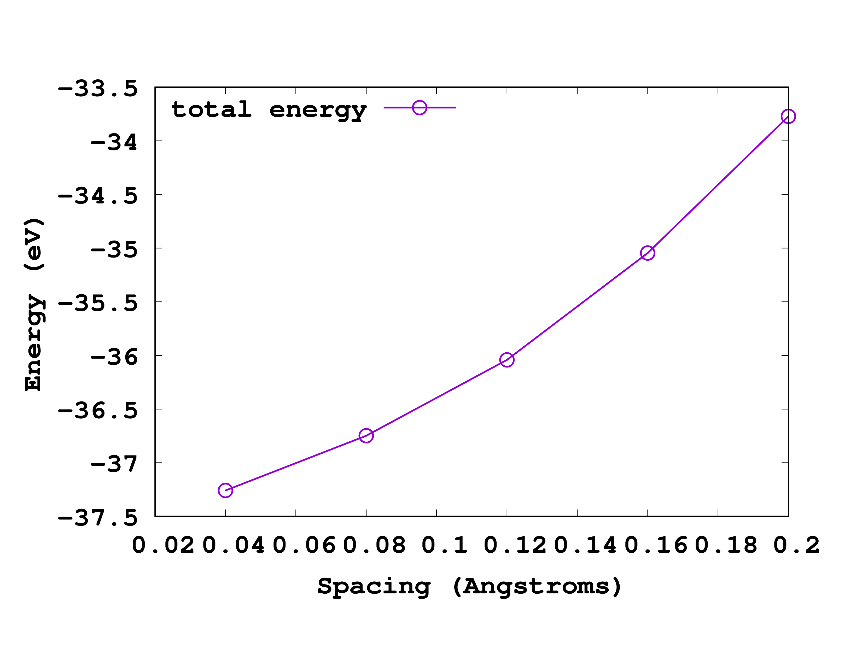
While the values are in reasonable agreement, there still present large deviations. This is because we employed here a too large grid spacing, uncapable of capturing the rapid change of the core charge around the nucleus. By reducing the grid spacing to a smaller value, one can converge the results of Octopus and recover the all-electron results from the NIST database.

The convergence of the total energy versus the grid spacing is illustrated in Fig. 1.

Especially for all-electron simulations, it can be worth to try using curvilinear coordinates. They are constructed such that the spacing is smaller near the atoms and larger far away from the atoms. This reduces the error with a smaller total number of points. This can be achieved by setting the variable “CurvMethod”.

We can set some additional variables to improve the convergence behavior:

Eigensolver = chebyshev_filter
OptimizeChebyshevFilterDegree = no
ChebyshevFilterLanczosOrder = 10
ChebyshevFilterDegree = 15
MaximumIter = 500

CurvMethod = curv_affine
#CurvMethod = curv_gygi
#CurvMethod = curv_modine
#CurvMethod = curv_briggs

Running this for a range of values for the spacing yields Fig. 2 for the convergence of the energy and Fig. 3 for the convergence of the eigenvalues of the states.

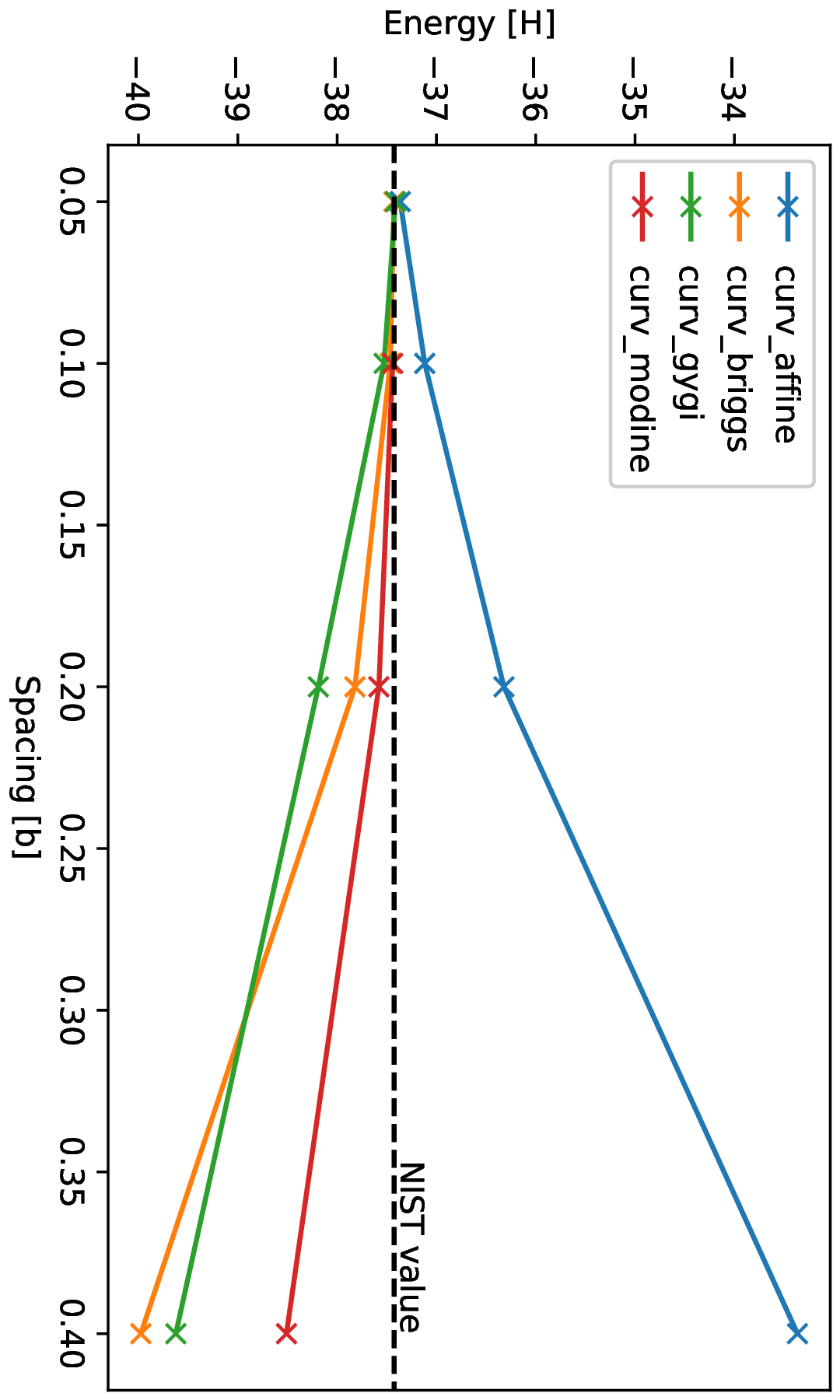
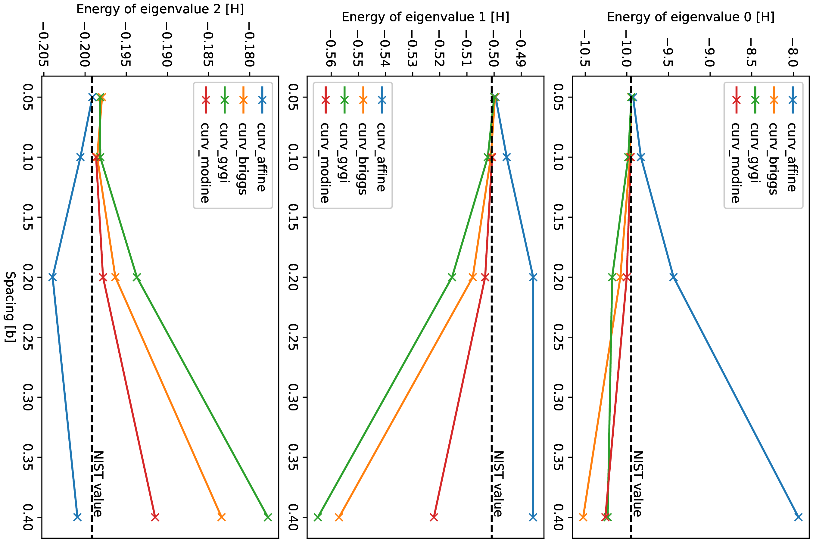
As one can see, the simulations with curvilinear grids approach the NIST values already at larger values of the spacing, thus using less grid points.

References