Light-induced orbital angular momentum

The orbital angular momentum of a system is often required to calculate different properties, for example circular dichroism ¹. For the Kohn-Sham system the expectation value of the angular momentum is given as

$\mathbf{L}(t) = \dfrac{1}{2} \int d\mathbf{r}\ \mathbf{r} \times \mathbf{j} (\mathbf{r},t) = -i \sum_k \int d\mathbf{r}\ \psi_k(\mathbf{r},t)\ (\mathbf{r} \times \mathbf{\nabla})\psi_k(\mathbf{r},t)$

In this tutorial we consider our system to be a small cluster of 7 Na atoms, a system that has been studied experimentally by many groups e.g.,².

Ground state

In order to calculate the time-dependent orbital angular momentum, first we need to obtain the ground state of the system.

Input

For this we use the following inp file.

CalculationMode = gs
UnitsOutput = eV_Angstrom

%Coordinates
 'Na' |  1.448679 | -2.605800 |  0.018588
 'Na' |  2.923505 |  0.571785 | -0.000212
 'Na' |  0.363003 |  2.955821 | -0.015874
 'Na' |  0.000000 |  0.000000 |  1.899415
 'Na' | -2.703005 |  1.253884 |  0.003526
 'Na' | -2.027140 | -2.178866 | -0.000901
 'Na' | -0.005043 |  0.003177 | -1.904541
%
PseudopotentialSet = hgh_lda

Extrastates = 2

Radius = 8.0*angstrom
Spacing = 0.5*angstrom

Eigensolver = chebyshev_filter

We notice that no XC functional is mentioned in the input which suggest that the DFT calculation will be done at the level of local density approximation (LDA).

Output

Running Octopus with the above input file will generate the converged ground state. The level of convergence can be checked at the last iteration step which looks like following.

*********************** SCF CYCLE ITER #   26 ************************
 etot  = -1.70208992E+01 abs_ev   =  4.80E-05 rel_ev   =  1.42E-06
 ediff =        1.74E-06 abs_dens =  3.95E-06 rel_dens =  5.64E-07
Matrix vector products:     25
Converged eigenvectors:      4

#  State  Eigenvalue [eV]  Occupation    Error
      1       -6.867103    2.000000   ( 6.9E-08)
      2       -4.027843    2.000000   ( 7.4E-08)
      3       -4.026091    2.000000   ( 7.3E-08)
      4       -3.889151    1.000000   ( 9.2E-08)
      5       -2.618515    0.000000   ( 1.7E-07)
      6       -1.578783    0.000000   ( 3.2E-04)

Density of states:

-------------------------------------%--------------------------------
-------------------------------------%--------------------------------
-------------------------------------%--------------------------------
-------------------------------------%--------------------------------
-------------------------------------%--------------------------------
%------------------------------------%-%---------------%-------------%
%------------------------------------%-%---------------%-------------%
%------------------------------------%-%---------------%-------------%
%------------------------------------%-%---------------%-------------%
%------------------------------------%-%---------------%-------------%
                                       ^


Elapsed time for SCF step    26:          1.22
**********************************************************************

Laser excitation

Using this converged ground state of Na7 cluster, we now can calculate the time-dependent generation of the orbital angular momentum due to excitation by a circularly polarized laser. For this we use the following inp file.

Input

CalculationMode = td
UnitsOutput = eV_Angstrom

%Coordinates
 'Na' |  1.448679 | -2.605800 |  0.018588
 'Na' |  2.923505 |  0.571785 | -0.000212
 'Na' |  0.363003 |  2.955821 | -0.015874
 'Na' |  0.000000 |  0.000000 |  1.899415
 'Na' | -2.703005 |  1.253884 |  0.003526
 'Na' | -2.027140 | -2.178866 | -0.000901
 'Na' | -0.005043 |  0.003177 | -1.904541
%
PseudopotentialSet = hgh_lda

Radius = 8.0*angstrom
Spacing = 0.5*angstrom

Extrastates = 0

Eigensolver = chebyshev_filter




TDPropagator = aetrs
TDExponentialMethod = lanczos
TDTimeStep = 0.05*fs   #0.0015*fs
TDPropagationTime = 20*fs

amplitude = 1e-2*eV/angstrom      # Amplitude of laser in volt/angstrom
omega = 3.75*eV                   # Frequency of laser in eV

%TDExternalFields
 electric_field | i | 1 | 0 | omega | "func"
%

tzero=TDPropagationTime*0.25
%TDFunctions
 "func" | tdf_from_expr | "amplitude*(sin(pi*(t/(2*tzero)))^2)*(t<=2*tzero)"
%

%TDOutput
 multipoles
 energy
 laser
 angular
%

The input file is very similar to the one discussed in Octopus Basics tutorial on the Time-dependent propagation. We notice that in this input file we ask octopus to write a TDOutput called angular which calculates the expectation value of the angular momentum of the Kohn-Sham system.

Output

Apart from the usual output that we observe in a typical Time-dependent propagation, the log file shows a block with the laser parameters:

******************* Time-dependent external fields *******************
 1:
   Electric Field.
   Polarization: ( 0.0000, 0.7071)( 0.7071, 0.0000)( 0.0000, 0.0000)
   Carrier frequency =     3.75000000 [eV]
   Envelope:
      Mode: time-dependent function parsed from the expression:
            f(t) = amplitude*(sin(pi*(t/(2*tzero)))^2)*(t<=2*tzero)
   Peak intensity       =      1.031025E-07 [a.u]
                        =      6.636095E+08 [W/cm^2]
   Int. intensity       =      1.598399E-05 [a.u]
   Fluence              =      2.931482E-06 [a.u]
   Ponderomotive energy =      6.773301E-06 [eV]
**********************************************************************

We find the time-dependence of the driving laser field, and of the response of the system by looking at the files lasers and multipoles in the td.general/ directory. They can be plotted using the following gnuplot scripts.

The external field

#set terminal qt persist enhanced font "Helvetica, 14"
#set encoding utf8

set t postscript enhanced color font "Monospace-Bold,25" landscape size 11,8.5
set output "laser.eps"

set xlabel "t  [ \U+210F/eV ]"
set ylabel "E(t)  [ V/\U+212B ]
plot [0:32] [-0.008:0.008] 'td.general/laser' u 2:3 w l lw 1.5 title "E_x", 'td.general/laser' u 2:4 w l lw 1.5 title "E_y"

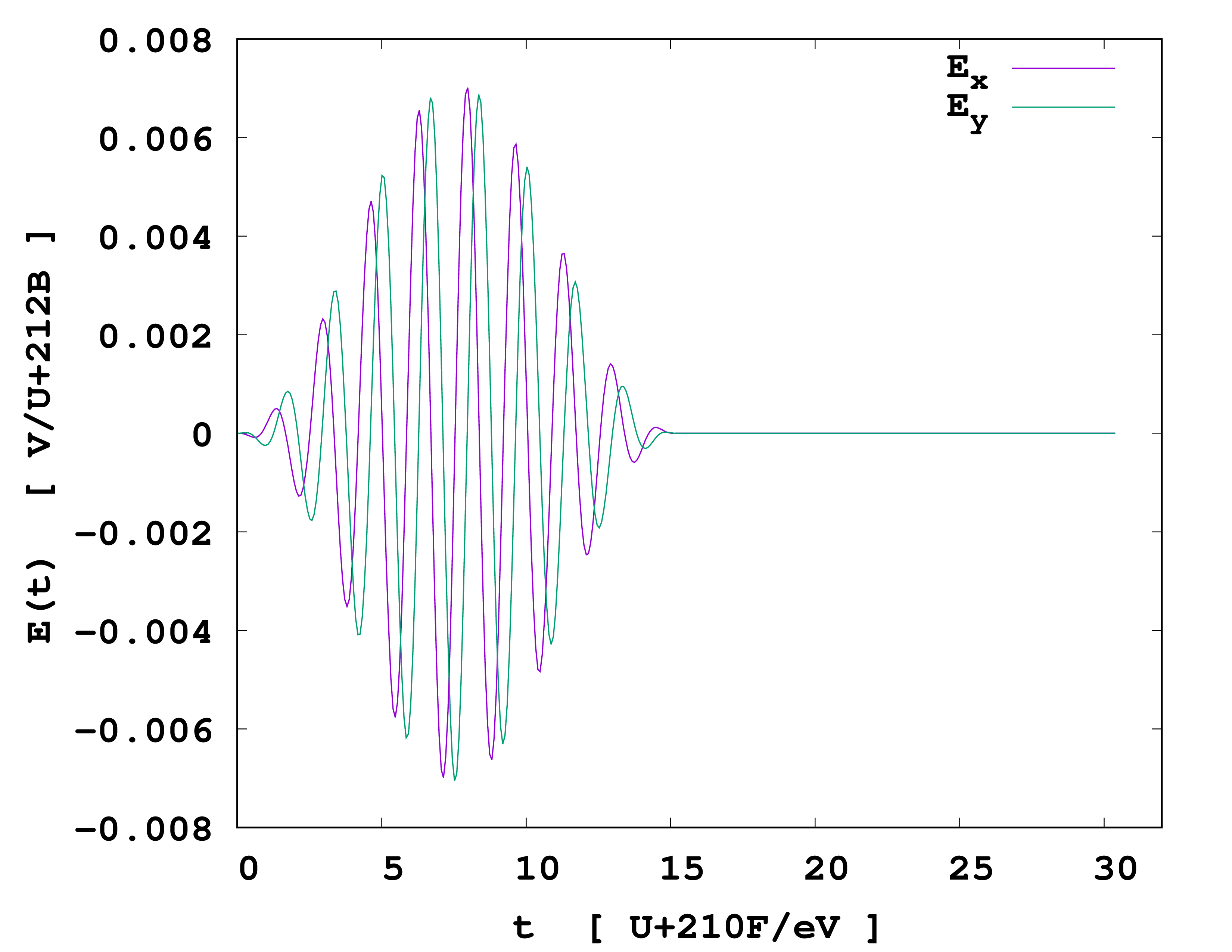
gives the time dependence of the laser field.

The induced dipole moment

#set terminal qt persist enhanced font "Helvetica, 14"
#set encoding utf8

set t postscript enhanced color font "Monospace-Bold,25" landscape size 11,8.5
set output "multipoles.eps"

set xlabel "t  [\U+210F/eV]"
set ylabel "p(t)  [\U+212B]"
plot [0:32] [-0.25:0.3] 'td.general/multipoles' u 2:4 w l lw 1.5 title "p_x", 'td.general/multipoles' u 2:5 w l lw 1.5 title "p_y"

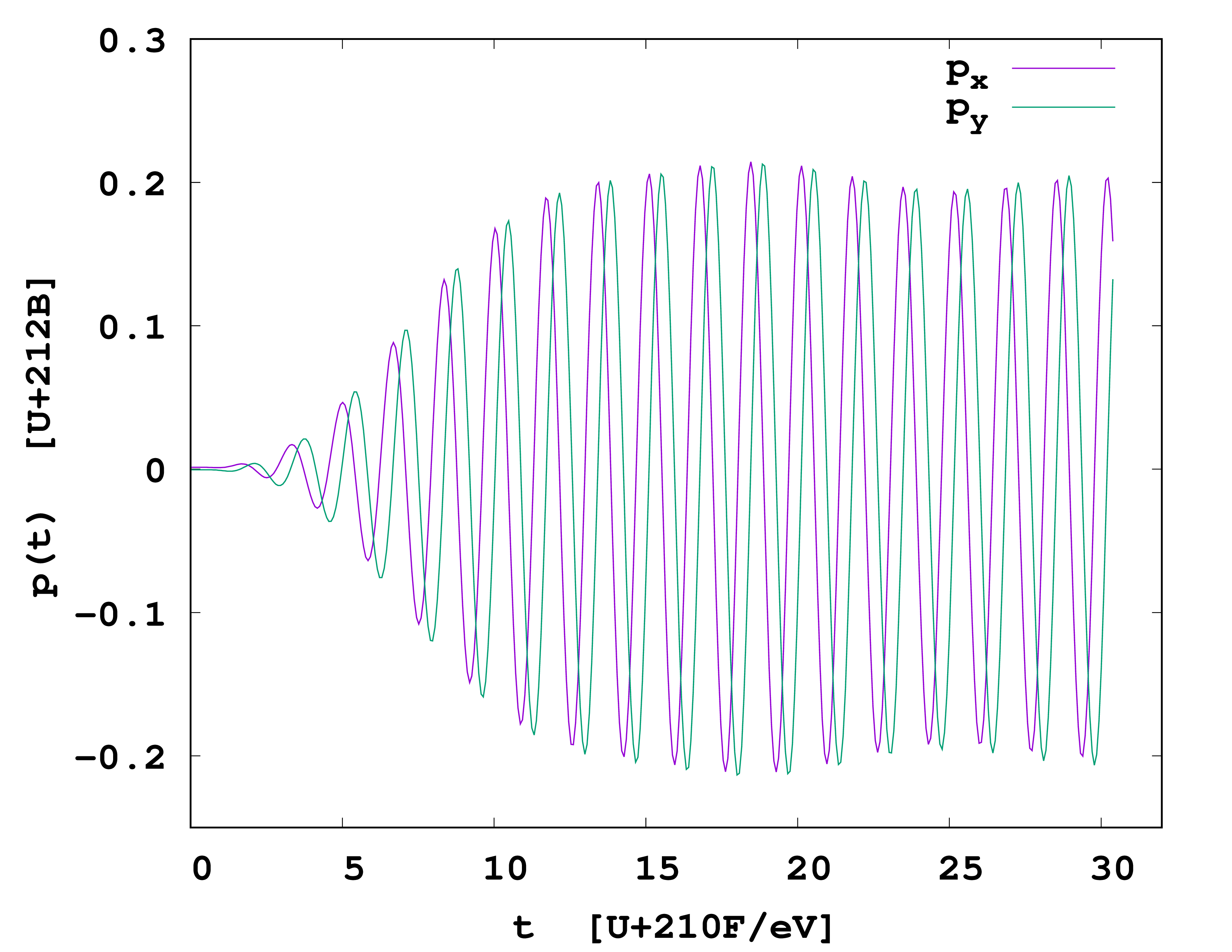
gives the time dependence of the laser field dipole moment.

We notice that the $x$- and $y$-component of the time dependent dipole moment increase with time and attains a saturation amplitude at the end of the laser pulse maintaining the same initial phase difference. Also, a careful comparison with the laser pulse reveals that for each of these components the dipole moment is phase-shifted by a quarter of a period with respect to the driving laser field, suggesting that the system is driven at a resonance frequency.

The induced magnetic moment

Finally, we can plot the data in the file td.general/angular using the following gnuplot script

#set terminal qt persist enhanced font "Helvetica, 14"
#set encoding utf8

set t postscript enhanced color font "Monospace-Bold,25" landscape size 11,8.5
set output "angular.eps"

set xlabel "t [\U+210F/eV]"
set ylabel "L(t) [ {/Symbol m}_B ]"
plot [0:32] [-0.0002:0.0085] 'td.general/angular' u 2:3 w l lw 2 title "L_x", 'td.general/angular' u 2:4 w l lw 2 title "L_y", 'td.general/angular' u 2:5 w l lw 3 title "L_z"

which gives the following result.

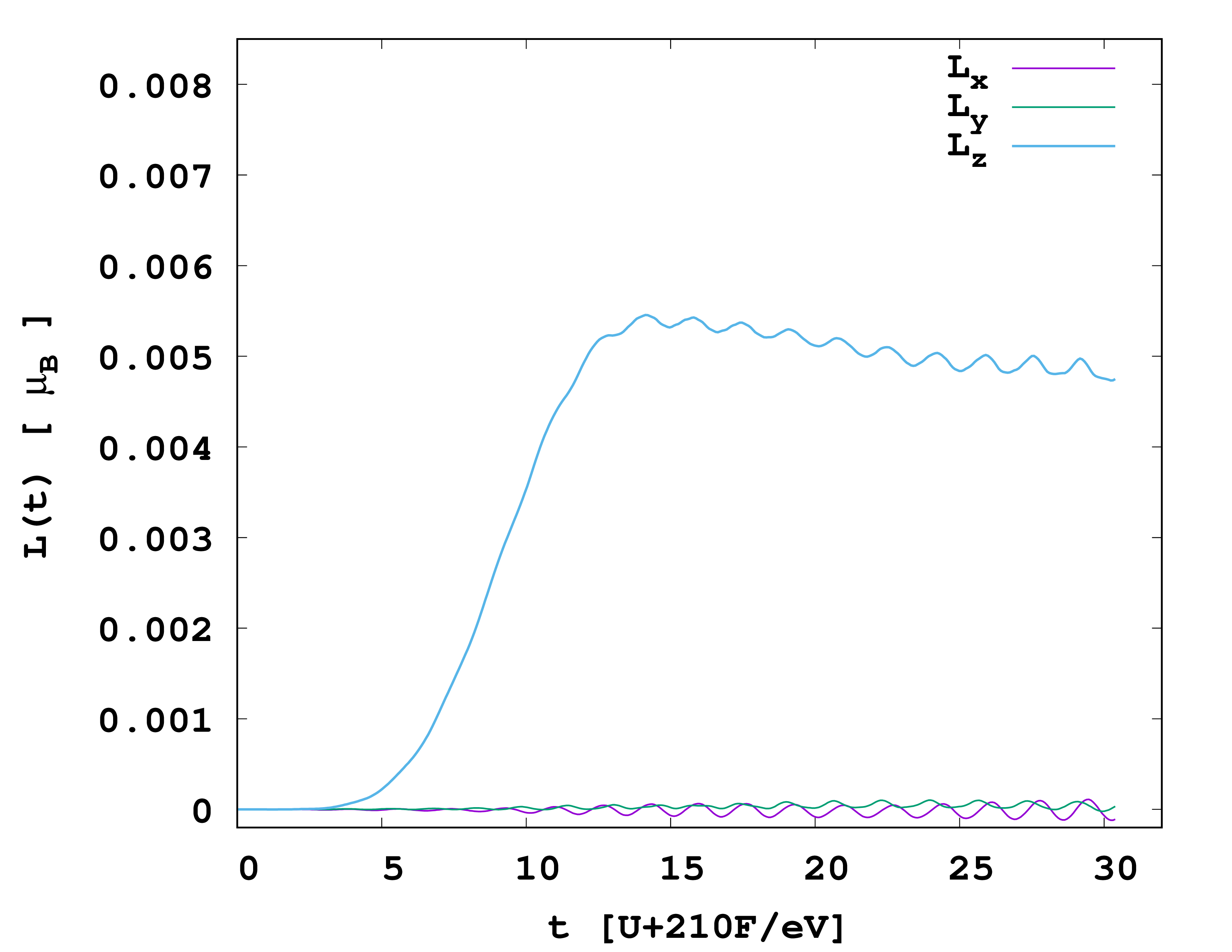
While the $x$- and $y$-component of the generated angular momentum $L(t)$ (expressed in terms of $\mu_B$) remains negligibly small the $z$-component increases with time as laser continues to pump energy and is saturated to a value a the end of the laser pulse. This result can be compared to the ones published in th reference ³, where the differences comes from the temporal profile of the laser pulse and the grid parameters.

Instead of asking octopus to calculate $L(t)$ directly, a nice exercise is to alternatively calculate ⁴ it from the time-dependent current-density ($\mathbf{j}(t)$) which can be obtained at chosen time intervals by using current in the variable block Output. This can be done using a bit of post-processing, e.g., as done in MagJell for calculating $L(t)$ in jellium spheres ⁴.

References